Waves in composites and metamaterials/Fresnel equations
< Waves in composites and metamaterialsThe content of these notes is based on the lectures by Prof. Graeme W. Milton (University of Utah) given in a course on metamaterials in Spring 2007.
A brief excursion into homogenization
One of the first questions that arise in the homogenization of composites is whether determining the effective behavior of the composite by some averaging process is the right thing to do. At this stage we ignore such questions and assume that there is a representative volume element (RVE) over which such an average can be obtained.
Let  be an average over some RVE of the -field at an atomic
scale. Similarly, let
be an average over some RVE of the -field at an atomic
scale. Similarly, let  be the average of the -field.
Recall, from the previous lecture, that the Maxwell equations have the form
(we have dropped the hats over the field quantities)
be the average of the -field.
Recall, from the previous lecture, that the Maxwell equations have the form
(we have dropped the hats over the field quantities)

For some conductors, at low frequencies, the permittivity tensor is given by
where  is the real part of the permittivity tensor and
  is the electrical conductivity tensor.
[1]
is the electrical conductivity tensor.
[1]
A mixture of conductors and dielectric materials may have properties which are quite different from those of the constituents. For example, consider the checkerboard material shown in Figure 1 containing an isotropic conducting material and an isotropic dielectric material.
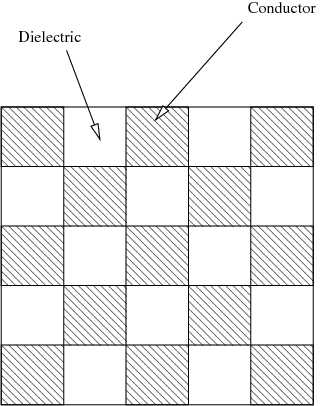 Figure 1. Checkerboard material containing conducting and dielectric phases. |
The conducting material has a permittivity of 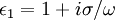 while the dielectric material has a permittivity of
  . The
effective permittivity of the checkerboard is given by
. The
effective permittivity of the checkerboard is given by

Plane waves
Let us assume that the material is isotropic. Then,

Therefore, we can write

The Maxwell equations then take the form

If we assume that  and
and  do not depend upon position, i.e.,
 and
and  , and
take the curl of equations (2), we get
, and
take the curl of equations (2), we get

Using the identity  ,
we get
,
we get

Since

we have

Therefore, from equation (3), we have

We can also write the above equations in the form

where  is the phase velocity (the velocity at which the wave crests
travel). To have a propagating wave, must be real. This will be the
case when and are both positive or both negative (see
Figure 2).
is the phase velocity (the velocity at which the wave crests
travel). To have a propagating wave, must be real. This will be the
case when and are both positive or both negative (see
Figure 2).
 Figure 2. Transparency and opacity of a material as a function of and . |
Let us look for plane wave solutions to the equations (4) of the form
where  and
and  is the wavelength. Then,
using the first of equations (2) we have
is the wavelength. Then,
using the first of equations (2) we have

where  .
.
Since  , we have (in terms of components with
respect to a orthonormal Cartesian basis)
, we have (in terms of components with
respect to a orthonormal Cartesian basis)
![\boldsymbol{\nabla} \cdot \mathbf{E} = \frac{\partial }{\partial x_m}\left[ E_{0m}~e^{i(k_l~x_l)}\right]
= i~k_l~\frac{\partial x_l}{\partial x_m}~E_{0m}~e^{i(k_l~x_l)}
= i~k_m~E_{0m}~e^{i(k_l~x_l)}
= i~(\mathbf{k}\cdot\mathbf{E}_0)~e^{i(\mathbf{k}\cdot\mathbf{x})} = 0 ~.](../I/m/bb3bf99fa22442f6275317581c254cc1.png)
Hence,

Similarly, since  , we have
![\boldsymbol{\nabla} \cdot \mathbf{H} = \cfrac{1}{\omega\mu}\left[
\frac{\partial }{\partial x_m}\left(\mathcal{E}_{mpq}~k_p~E_{0q}~e^{i(k_l~x_l)}\right)
\right]
= \cfrac{i}{\omega\mu}\left[\mathcal{E}_{mpq}~k_p~E_{0q}~k_m~e^{i(k_l~x_l)}
\right]
= \cfrac{i}{\omega\mu}~\mathbf{k}\cdot(\mathbf{k}\times\mathbf{E}_0)~e^{i(\mathbf{k}\cdot\mathbf{x})}~.](../I/m/44d6f1be880607073dec4e75a1820d30.png)
Hence,

Plugging equation (5) into the first of equations (4) we get
![\begin{align}
\left[\nabla^2 \mathbf{E} + \kappa^2~\mathbf{E}(\mathbf{x})\right]_n & =
\frac{\partial }{\partial x_m}\left[\frac{\partial }{\partial x_m}\left(
E_{0n}~e^{i k_l x_l}\right)\right] + \kappa^2~E_{0n}~
e^{i k_l x_l} \\
& =
\frac{\partial }{\partial x_m}\left[E_{0n}~\left(i~k_l~\frac{\partial x_l}{\partial x_m}\right)~
e^{i k_l x_l}\right] + \kappa^2~E_{0n}~
e^{i k_l x_l} \\
& =
i~E_{0n}~k_m~\frac{\partial }{\partial x_m}\left(e^{i k_l x_l}\right) +
\kappa^2~E_{0n}~
e^{i k_l x_l} \\
& =
i~E_{0n}~k_m~\left(i~k_l~\frac{\partial x_l}{\partial x_m}\right)~e^{i k_l x_l} +
\kappa^2~E_{0n}~
e^{i k_l x_l} \\
& =
- E_{0n}~k_m~k_m~e^{i k_l x_l} +
\kappa^2~E_{0n}~e^{i k_l x_l} ~.
\end{align}](../I/m/a7a13c4329854ebe60a93761960e0145.png)
Reverting back to Gibbs notation, we get

Therefore,

Plugging the solution (6) into the second of equations (4) (and using index notation as before) we get
![\begin{align}
\left[\nabla^2 \mathbf{H} + \kappa^2~\mathbf{H}(\mathbf{x})\right]_n & =
\cfrac{1}{\omega\mu}\left\{
\frac{\partial }{\partial x_m}\left[\frac{\partial }{\partial x_m}\left(
\mathcal{E}_{npq}~k_p~E_{0q}~e^{i k_l x_l}\right)\right] + \kappa^2~
\mathcal{E}_{npq}~k_p~E_{0q}~e^{i k_l x_l}\right\} \\
& =
\cfrac{1}{\omega\mu}\left\{
\frac{\partial }{\partial x_m}
\left[\mathcal{E}_{npq}~k_p~E_{0q}~\left(i~k_l~\frac{\partial x_l}{\partial x_m}\right)~
e^{i k_l x_l}\right] + \kappa^2~
\mathcal{E}_{npq}~k_p~E_{0q}~e^{i k_l x_l}\right\} \\
& =
\cfrac{1}{\omega\mu}\left\{
i~\mathcal{E}_{npq}~k_p~k_m~E_{0q}~\left[i~k_l~\frac{\partial x_l}{\partial x_m}\right]~
e^{i k_l x_l} + \kappa^2~
\mathcal{E}_{npq}~k_p~E_{0q}~e^{i k_l x_l}\right\} \\
& =
\cfrac{1}{\omega\mu}\left\{
- \mathcal{E}_{npq}~k_p~k_m~k_m~E_{0q}~e^{i k_l x_l} + \kappa^2~
\mathcal{E}_{npq}~k_p~E_{0q}~e^{i k_l x_l}\right\}
\end{align}](../I/m/a793d0616b0f4f24bdbc06130a1552c6.png)
In Gibbs notation, we then have

Therefore, once again, we get
Reflection at an Interface
The following is based on the description given in [Lorrain88]. Figure 3 shows an electromagnetic wave that is incident upon an interface separating two mediums.
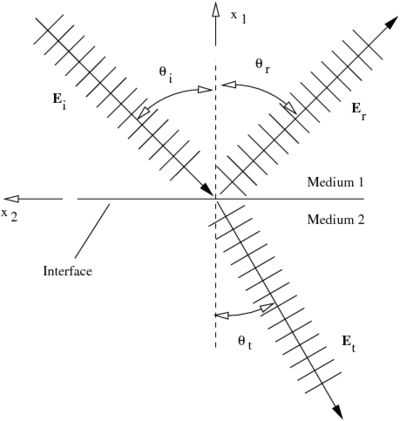 Figure 3. Reflection of an electromagnetic wave at an interface. |
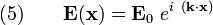
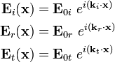
We ignore the time-dependent component of the electric fields and assume that we can express the waves shown in Figure 3 in the form
where  are the wave vectors.
Since the oscillations at the interface must have the same period (the requirement of continuity), we must have

This means that the tangential components of must
be equal at the interface. Therefore,

Now,
where  and
and  are the phase velocities in medium 1 and medium 2,
respectively. Hence we have,
are the phase velocities in medium 1 and medium 2,
respectively. Hence we have,
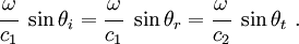
This implies that
The refractive index is defined as

where  is the phase velocity is vacuum. Therefore, we get
Polarized wave with the  parallel to the plane of incidence
Consider the  -polarized wave shown in Figure 4. The
figure represents an infinite wave polarized with the vector
polarized parallel to the plane of incidence. This is also called the
TM (transverse magnetic) case.
-polarized wave shown in Figure 4. The
figure represents an infinite wave polarized with the vector
polarized parallel to the plane of incidence. This is also called the
TM (transverse magnetic) case.
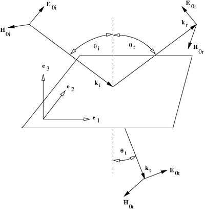 Figure 4. Infinite wave polarized with the -vector parallel to the plane of incidence. |
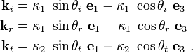
Let us define

Recall that,
Let us choose an orthonormal basis ( ) such that
the
) such that
the  vector lies on the interface and is parallel the plane of
incidence. The
vector lies on the interface and is parallel the plane of
incidence. The  vector lies on the plane of incidence and the
 vector is normal to the interface. Then the vectors
  ,
,
 , and
, and  may be expressed in this basis as
Similarly, defining

we get
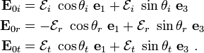
Using the definition
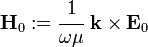
we then get
Hence, with the vector  expressed as
 , we get
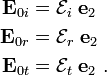
![\begin{align}
\mathbf{E}_i(\mathbf{x}) & =
(\mathcal{E}_i~\cos\theta_i~\mathbf{e}_1 + \mathcal{E}_i~\sin\theta_i~\mathbf{e}_3)
~e^{i[\kappa_1(x_1\sin\theta_i - x_3\cos\theta_i)]} \\
\mathbf{E}_r(\mathbf{x}) & =
(-\mathcal{E}_r~\cos\theta_r~\mathbf{e}_1 + \mathcal{E}_r~\sin\theta_r~\mathbf{e}_3)
~e^{i[\kappa_1(x_1\sin\theta_r + x_3\cos\theta_r)]} \\
\mathbf{E}_t(\mathbf{x}) & =
(\mathcal{E}_t~\cos\theta_t~\mathbf{e}_1 + \mathcal{E}_t~\sin\theta_t~\mathbf{e}_3)
~e^{i[\kappa_2(x_1\sin\theta_t - x_3\cos\theta_t)]}~.
\end{align}](../I/m/4d743a3b2d973c067c4dbb2ff9a5afaa.png)
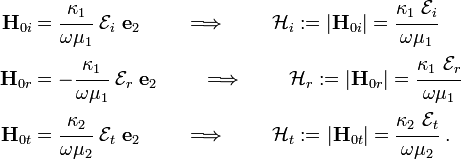
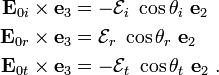
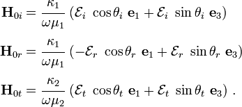
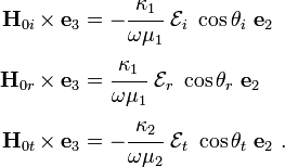
Similarly,
![\begin{align}
\mathbf{H}_i(\mathbf{x}) & = -\mathcal{H}_i~\mathbf{e}_2~
~e^{i[\kappa_1(x_1\sin\theta_i - x_3\cos\theta_i)]} \\
\mathbf{H}_r(\mathbf{x}) & = -\mathcal{H}_r~\mathbf{e}_2~
~e^{i[\kappa_1(x_1\sin\theta_r + x_3\cos\theta_r)]} \\
\mathbf{H}_t(\mathbf{x}) & = -\mathcal{H}_t~\mathbf{e}_2~
~e^{i[\kappa_2(x_1\sin\theta_t - x_3\cos\theta_t)]}~.
\end{align}](../I/m/84342e42f4395629f6630d3bc0d6d808.png)
At the interface, continuity requires that the tangential components of
the vectors and  are continuous. Clearly, from the above
equations, the
are continuous. Clearly, from the above
equations, the  vectors are tangential to the interface. Also,
at the interface
vectors are tangential to the interface. Also,
at the interface  and
and  is arbitrary. Hence, continuity
of the components of at the interface can be achieved if
is arbitrary. Hence, continuity
of the components of at the interface can be achieved if

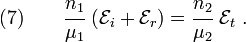
In terms of the electric field, we then have
Recall that the refractive index is given by 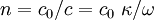 .
Therefore, we can write the above equation as
.
Therefore, we can write the above equation as
The tangential components of the vectors at the interface are given
by  . Therefore, the tangential components of the
 vectors at the interface are
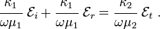
Using the arbitrariness of and from the continuity of the
vectors at the interface, we have

Since  , we have

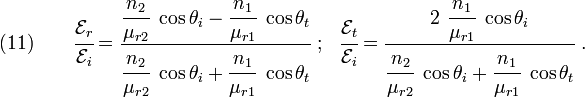
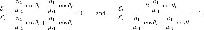
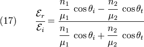
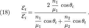
From equations (7) and (8), we get two more relations:
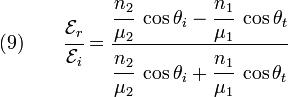
and
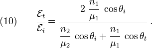
Equations (7), (8), (9),
and (10) are the Fresnel equations for -polarized
electromagnetic waves.
If we define,
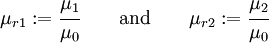
where  is the permeability of vacuum, then we can write equations
(9) and (10) as
is the permeability of vacuum, then we can write equations
(9) and (10) as
Note that
For non-magnetic materials we have 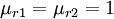 . Hence,
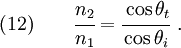
Also, from Snell's law
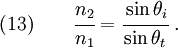
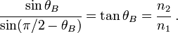
Combining equations (12) and (13), we get

If  we have
  . Hence,

This is the condition that defines Brewster's angle
( ). Plugging
equation (14) into equation (13), we get
). Plugging
equation (14) into equation (13), we get
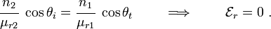
This relation can be used to solve for Brewster's angle for various media. At Brewster's angle, we have
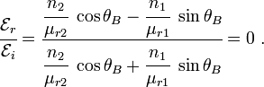
Hence, the sign of  changes at the Brewster angle.
Also, note that if  and
and  , since
 we must have
  . Then,
by Snell's law
. Then,
by Snell's law
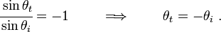
Hence,
So the radiation is transmitted at the angle  and
none is reflected.
and
none is reflected.
More can be said about the matter. In fact, an interface separating media
with and "behaves like a
mirror". Consider the interface in Figure 5. Suppose that
on the left side of the mirror, and solve Maxwell's
equations

Let the solution be of the form
![\mathbf{E}(\mathbf{x}) = [E_1(\mathbf{x}), E_2(\mathbf{x}), E_3(\mathbf{x})] ~~\text{and}~~
\mathbf{H}(\mathbf{x}) = [H_1(\mathbf{x}), H_2(\mathbf{x}), H_3(\mathbf{x})] ~.](../I/m/27587347cc5ce9ae08caf83e22c71d2d.png)
Suppose that the right hand side of the interface has reflected fields, i.e.,
![\begin{align}
\mathbf{E}(\mathbf{x}) & = [-E_1(-x_1,x_2,x_3), E_2(-x_1,x_2,x_3),
E_3(-x_1,x_2,x_3)] ~~\text{and}~~ \\
\mathbf{H}(\mathbf{x}) & = [-H_1(-x_1,x_2,x_3), H_2(-x_1,x_2,x_3),
H_3(-x_1,x_2,x_3)] ~.
\end{align}](../I/m/d199304f429e046862017ae3dcaa8525.png)
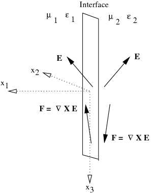 Figure 5. Reflection at an interface due to negative and . |
Also, on the right hand side, let
![\boldsymbol{\nabla} \times \mathbf{E} = [F_1(\mathbf{x}), F_2(\mathbf{x}), F_3(\mathbf{x})] ~.](../I/m/16a96a7b11016dcfb0e9d5d6d68231a9.png)
Then, to the right of the interface, we have
![\begin{align}
\boldsymbol{\nabla} \times \mathbf{E} = & \left\{
\left[\frac{\partial }{\partial x_2}[E_3(-x_1,x_2,x_3)] -
\frac{\partial }{\partial x_3}[E_2(-x_1,x_2,x_3)]\right],\right. \\
&
\left[-\frac{\partial }{\partial x_3}[E_1(-x_1,x_2,x_3)] +
\frac{\partial }{\partial x_1}[E_3(-x_1,x_2,x_3)]\right], \\
& \left.
\left[-\frac{\partial }{\partial x_1}[E_2(-x_1,x_2,x_3)] +
\frac{\partial }{\partial x_2}[E_1(-x_1,x_2,x_3)]\right]\right\}
\end{align}](../I/m/fb120c31286cba7afffd1de1b93e8a32.png)
or,
![\boldsymbol{\nabla} \times \mathbf{E} = [F_1(-x_1,x_2,x_3), -F_2(-x_1,x_2,x_3), -F_3(x_1,x_2,x_3)]~.](../I/m/386eede79bf7c4ab32ea582f293c5569.png)
Polarized wave with the perpendicular to the plane of incidence
For a plane polarized wave with the vector perpendicular to the
plane of incidence, we have
Therefore,
Continuity of tangential components of at the interface gives

The tangential components of at the interface are given by
From continuity at the interface and using the arbitrariness of , we
get (from the above equations with )

Using the relation  , we get

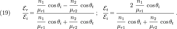
From equations (15) and (16), we get
and
Equations (15), (16), (17), and (18) are the Fresnel equations a wave polarized with the vector perpendicular to the plane of incidence. We may also
write the last two equations as
From the above equations, there is no reflected wave only if
This is only possible if there is no interface. Therefore, in the presence of a interface, there is always a reflected wave for this situation.
Footnotes
- ↑ The above relation for the permittivity tensor can be obtained as follows.
Recall that
 and the electric displacement
 are related to the electric field by


References
[Lorrain88]
P. Lorrain, D. R. Corson, and F. Lorrain. Electromagnetic fields and waves: including electric circuits. Freeman, New York, 1988.