Waves in composites and metamaterials/Elastodynamics and electrodynamics
< Waves in composites and metamaterialsThe content of these notes is based on the lectures by Prof. Graeme W. Milton (University of Utah) given in a course on metamaterials in Spring 2007.
Dissipation
Recall from the previous lecture that the average rate of work done in a cycle of oscillation of material with frequency dependent mass is
![\begin{align}
\mathcal{P} & = \cfrac{\omega}{2~\pi}
\int_{0}^{2\pi/\omega}~\mathbf{F}(t)\cdot\mathbf{V}(t)~\text{d}t \\
& = \cfrac{\text{Re}(\widehat{\mathbf{F}})\cdot\text{Re}(\widehat{\mathbf{V}}) +
\text{Im}(\widehat{\mathbf{F}})\cdot\text{Im}(\widehat{\mathbf{V}})}{2} \\
& = \omega~[\text{Re}(\widehat{\mathbf{V}})\cdot\text{Im}[\boldsymbol{M}(\omega)]\cdot\text{Re}(\widehat{\mathbf{V}}) +
\text{Im}(\widehat{\mathbf{V}})\cdot\text{Im}[\boldsymbol{M}(\omega)]\cdot\text{Im}(\widehat{\mathbf{V}})].
\end{align}](../I/m/ad8c5c606e6fecb443ed3f09fde4bccb.png)
This quadratic form will be non-negative for all choices of  if
and only if
if
and only if  is positive semidefinite for all real
 . Therefore, a restriction on the behavior of such materials
is that
. Therefore, a restriction on the behavior of such materials
is that
![{
\text{Im}[\boldsymbol{M}(\omega)] \ge 0 ~.
}](../I/m/4269d20dcb79f42558b02618f20b8a4f.png)
Similarly, for electrodynamics, the average power dissipated into heat is given by
![\text{(1)} \qquad
\mathcal{P} = \cfrac{\omega}{2~\pi}
\int_{0}^{2\pi/\omega}~\left[\mathbf{E}(t)\cdot\frac{\partial \mathbf{D}(t)}{\partial t} +
\mathbf{H}(t)\cdot\frac{\partial \mathbf{B}(t)}{\partial t}\right]~dt ~.](../I/m/df49ef48115b423c42b5379240324283.png)
In this case, the quantity  is equivalent to the voltage and the
quantity rate of change of electrical displacement
is equivalent to the voltage and the
quantity rate of change of electrical displacement  is equivalent to the current (recall that in electrostatics the power is
given by
is equivalent to the current (recall that in electrostatics the power is
given by  ). In addition, we also have a contribution due to
magnetic induction.
). In addition, we also have a contribution due to
magnetic induction.
Let us assume that the fields can be expressed in harmonic form, i.e.,
![\mathbf{E}(t) = \text{Re}[\widehat{\mathbf{E}}~e^{-i\omega t}] ~;~~
\mathbf{H}(t) = \text{Re}[\widehat{\mathbf{H}}~e^{-i\omega t}]](../I/m/ee131b7b9f8047c1c61c17b6b67a46b2.png)
or equivalently as

Also, recall that,

Therefore, for real  and real
  , we can write equation
(1) as (with the substitution
, we can write equation
(1) as (with the substitution  ),
),
![\begin{align}
\mathcal{P} = \cfrac{\omega}{2~\pi}
\int_{0}^{2\pi}~ &
\left[\text{Re}(\widehat{\mathbf{E}})~\cos z + \text{Im}(\widehat{\mathbf{E}})~\sin z\right]\cdot
\left\{\text{Im}(\boldsymbol{\epsilon})\cdot
\left[\text{Re}(\widehat{\mathbf{E}})~\cos z + \text{Im}(\widehat{\mathbf{E}})~\sin z\right]\right\} + \\
&
\left[\text{Re}(\widehat{\mathbf{H}})~\cos z + \text{Im}(\widehat{\mathbf{H}})~\sin z\right]\cdot
\left\{\text{Im}(\boldsymbol{\mu})\cdot
\left[\text{Re}(\widehat{\mathbf{H}})~\cos z + \text{Im}(\widehat{\mathbf{H}})~\sin z\right]\right\}~\text{d}z
\end{align}](../I/m/ae19752785e106c59b4a36ef924b69f2.png)
Expanding out, and using the fact that

we have,
![\text{(2)} \qquad
\mathcal{P} = \cfrac{\omega}{2}
\left[\text{Re}(\widehat{\mathbf{E}})\cdot\text{Im}(\boldsymbol{\epsilon})\cdot\text{Re}(\widehat{\mathbf{E}}) +
\text{Im}(\widehat{\mathbf{E}})\cdot\text{Im}(\boldsymbol{\epsilon})\cdot\text{Im}(\widehat{\mathbf{E}}) +
\text{Re}(\widehat{\mathbf{H}})\cdot\text{Im}(\boldsymbol{\mu})\cdot\text{Re}(\widehat{\mathbf{H}}) +
\text{Im}(\widehat{\mathbf{H}})\cdot\text{Im}(\boldsymbol{\mu})\cdot\text{Im}(\widehat{\mathbf{H}})\right] ~.](../I/m/3711e2e7986ef7ff3685e841eb7e0253.png)
Since  and the power
  , the quadratic forms in
equation (2) require that
, the quadratic forms in
equation (2) require that

Note that if the permittivity is expressed as
the requirement  implies that the conductivity
  .
Therefore, if the conductivity is greater than zero, there will be
dissipation.
.
Therefore, if the conductivity is greater than zero, there will be
dissipation.
Brief introduction to elastodynamics
A concise introduction to the theory of elasticity can be found in Atkin80. In this section, we consider the linear theory of elasticity for infinitesimal strains and small displacements.
Consider the body ( ) shown in Figure~1. Let
  be a subpart of the body (in the interior of or sharing a
part of the surface of ). Postulate the existence of a force
be a subpart of the body (in the interior of or sharing a
part of the surface of ). Postulate the existence of a force
 per unit area on the surface of where
  is
the outward unit normal to the surface of . Then
is
the outward unit normal to the surface of . Then  is the
force exerted on by the material outside or by surface
tractions.
is the
force exerted on by the material outside or by surface
tractions.
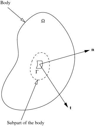 Figure 1. Illustration of the concept of stress. |
From the balance of forces on a small tetrahedron (), we can show
that is linear in . Therefore,

where  is a second-order tensor called the stress tensor.
Since the tetrahedron cannot rotate at infinite velocity as its size goes to zero (conservation of angular momentum), we can show that the stress tensor is symmetric, i.e.,

In particular, for a fluid,

where  is the pressure.
Let us assume that the stress depends only on the strain (and not on strain gradients or strain rates), where the strain is defined as
![\text{(3)} \qquad
\boldsymbol{\epsilon} = \frac{1}{2}\left[\boldsymbol{\nabla}\mathbf{u} + (\boldsymbol{\nabla}\mathbf{u})^T\right] ~.](../I/m/d8c71a7fa9e4518356d6fd258d8baed4.png)
Here  is the displacement field. Note that a gradient of the
displacement field is used to define the strain because rigid body motions
should not affect and a rigid body rotation gives zero strains
(for small displacements).
is the displacement field. Note that a gradient of the
displacement field is used to define the strain because rigid body motions
should not affect and a rigid body rotation gives zero strains
(for small displacements).
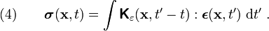
Assume that depends linearly on  so that
![\boldsymbol{\sigma}(\mathbf{x},t) = \int \text{d}\mathbf{x}'~
\left[\int \boldsymbol{\mathsf{K}}_{\varepsilon}(\mathbf{x},\mathbf{x}',t' - t):\boldsymbol{\epsilon}(\mathbf{x},t')~\text{d}t'\right] ~.](../I/m/c44a3fc4995bbf5a2d65831c62ff2927.png)
Note that this assumption ignores preexisting internal stresses such as those found in prestressed concrete. If the material can be approximated as being local, then
Taking the Fourier transforms of equation (4), we get

where
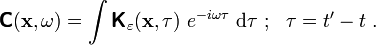
In index notation, equation (5) can be written as
Causality implies that stresses at time  can only depend on strains of
previous times, i.e., if
can only depend on strains of
previous times, i.e., if  or
or  . Therefore,

This in turn implies that the integral converges only if  ,
i.e.,
,
i.e.,  is analytic when .
In the absence of body forces, the equation of motion of the body can be written as
where  is the mass density,
  is the internal force
per unit volume, and
is the internal force
per unit volume, and  is the acceleration.
Hence, this is just the expression of Newton's second law for continuous
systems.
is the acceleration.
Hence, this is just the expression of Newton's second law for continuous
systems.
For a material which has a frequency dependent mass, equation (6) may be written as
where causality implies that if  then
then  .
.
Taking the Fourier transform of equation (7), we get

Substituting equation (5) into equation (8) we get

Also, taking the Fourier transform of equation (3), we have
![\text{(10)} \qquad
\widehat{\boldsymbol{\epsilon}} = \frac{1}{2}\left[\boldsymbol{\nabla} \widehat{\mathbf{u}} + (\boldsymbol{\nabla} \widehat{\mathbf{u}})^T\right] ~.](../I/m/646611d289a8b0c78d64a06263017807.png)
Since  and
and  are symmetric, we must have
Because of this symmetry, we can replace by  in
equation (9) to get
in
equation (9) to get

Dropping the hats, we then get the wave equation for elastodynamics

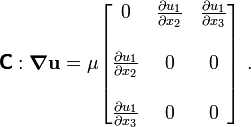
Antiplane shear
Let us now consider the case of antiplane shear. Assume that  is
isotropic, i.e.,
is
isotropic, i.e.,
![\boldsymbol{\mathsf{C}}:\boldsymbol{\nabla}\mathbf{u} = \mu~[\boldsymbol{\nabla}\mathbf{u} + (\boldsymbol{\nabla}\mathbf{u})^T] + \lambda~\text{tr}(\boldsymbol{\nabla}\mathbf{u})~\boldsymbol{\mathit{1}}](../I/m/2a922a685453440c8a24381c7ad33d29.png)
where  is the shear modulus and
  is the Lame modulus.
Let us assume that and are independent of  , i.e.,

Let us look for a solution with  and
and  independent of
, i.e.,
independent of
, i.e.,  . This is an out of plane mode of
deformation.
. This is an out of plane mode of
deformation.
Then, noting that 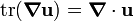 , we have
Therefore,
![[\boldsymbol{\mathsf{C}}:\boldsymbol{\nabla}\mathbf{u}]_{ij} =
\mu~\left[\frac{\partial u_i}{\partial x_j} + \frac{\partial u_j}{\partial x_i}\right]](../I/m/2b5daee58b921c080e82c028eb46daa6.png)
or
Therefore
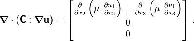
Plugging into the wave equation (11) we get
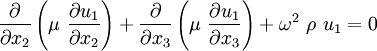
or (using the two-dimensional gradient operator  )
)

TM and TE modes in electromagnetism
Let us now consider the TM (transverse magnetic field) and TE (transverse electric field) modes in electromagnetism and look for parallels with antiplane shear in elastodynamics.
Recall the Maxwell equations (with hats dropped)

Assume that and  are scalars which are independent of ,
i.e.,
are scalars which are independent of ,
i.e., 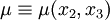 and
and  .
.
For the TE case, we look for solutions with  and
and  independent of , i.e.,
  .
.
Then,
![\boldsymbol{\nabla} \times \mathbf{E} = \left[0, \frac{\partial E_1}{\partial x_3}, - \frac{\partial E_1}{\partial x_2}\right]~.](../I/m/06b58a7799dd6df934005a53ffb9e594.png)
This implies that
![\mathbf{H} = \left[ 0, \cfrac{1}{i\omega\mu}~\frac{\partial E_1}{\partial x_3},
- \cfrac{1}{i\omega\mu}~\frac{\partial E_1}{\partial x_2}\right]~.](../I/m/268c706bae38121b240cd94370e8282c.png)
Therefore,
![\boldsymbol{\nabla} \times \mathbf{H} = \left[
-\frac{\partial }{\partial x_3}\left(\cfrac{1}{i\omega\mu}~\frac{\partial E_1}{\partial x_3}\right)
-\frac{\partial }{\partial x_2}\left(\cfrac{1}{i\omega\mu}~\frac{\partial E_1}{\partial x_2}\right),
0, 0\right]~.](../I/m/8f8acdebcc995ecf51eb3b6fc5a1e6de.png)
or,
![\boldsymbol{\nabla} \times \mathbf{H} = \cfrac{i}{\omega}\left[
\frac{\partial }{\partial x_2}\left(\cfrac{1}{\mu}~\frac{\partial E_1}{\partial x_2}\right) +
\frac{\partial }{\partial x_3}\left(\cfrac{1}{\mu}~\frac{\partial E_1}{\partial x_3}\right),
0, 0\right]
= \cfrac{i}{\omega} \left[\overline{\boldsymbol{\nabla}} \cdot\left(\cfrac{1}{\mu(x_2,x_3)}
\overline{\boldsymbol{\nabla}} E_1\right), 0, 0\right] ~.](../I/m/cc4e1692b57dbf191f9430fdeded53bd.png)
Plugging into equation (13) we get the TE equation
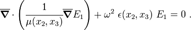
This equation has the same form as equation (12).
More generally, if
![\boldsymbol{\mu} = \boldsymbol{\mu}(x_2,x_3) =
\begin{bmatrix}
\mu_{11} & 0 & 0 \\ 0 & \mu_{22} & \mu_{23} \\ 0 & \mu_{23} & \mu_{33}
\end{bmatrix} =
\begin{bmatrix}
\mu_{11} & \left[\mathsf{0}\right] \\ \left[\mathsf{0}\right] & \left[\mathsf{M}\right]
\end{bmatrix}
\quad \text{where} \quad
\left[\mathsf{M}\right] =
\begin{bmatrix}
\mu_{22} & \mu_{23} \\ \mu_{23} & \mu_{33}
\end{bmatrix} \equiv \boldsymbol{M}](../I/m/54262925b09b9019fd6db3a0a9cd225b.png)
and
![\boldsymbol{\epsilon} = \boldsymbol{\epsilon}(x_2,x_3) =
\begin{bmatrix}
\epsilon_{11} & \left[\mathsf{0}\right] \\ \left[\mathsf{0}\right] & \left[\mathsf{N}\right]
\end{bmatrix}
\quad \text{where} \quad
\left[\mathsf{N}\right] =
\begin{bmatrix}
\epsilon_{22} & \epsilon_{23} \\ \epsilon_{23} & \epsilon_{33}
\end{bmatrix} \equiv \boldsymbol{N}](../I/m/6c597e517a5a02c1604f3cd0c21d4b9e.png)
we get the TE equation
![{
\overline{\boldsymbol{\nabla}} \cdot\left[\left(\boldsymbol{R}_{\perp}\cdot\boldsymbol{M}^{-1}\cdot\boldsymbol{R}_{\perp}^T\right)\cdot
\overline{\boldsymbol{\nabla}} E_1\right] + \omega^2~\epsilon_{11}~E_1~\mathbf{1} = \mathbf{0}
}
\qquad \text{where} \qquad
\boldsymbol{R}_{\perp} \equiv \left[\mathsf{R}\right]_{\perp} =
\begin{bmatrix} 0 & 1 \\ -1 & 0 \end{bmatrix} ~.](../I/m/c479841432fee69d4252e1c5b1b6cc74.png)
Similarly, there is a TM equation with  of the form
![{
\overline{\boldsymbol{\nabla}} \cdot\left[\left(\boldsymbol{R}_{\perp}\cdot\boldsymbol{N}^{-1}\cdot\boldsymbol{R}_{\perp}^T\right)
\cdot\overline{\boldsymbol{\nabla}} H_1\right] + \omega^2~\mu_{11}~H_1~\mathbf{1} = \mathbf{0}
}](../I/m/1431c2e1c698fd7b3b89681a5f90308b.png)
which for the isotropic case reduces to
The general solution independent of is a superposition of the TE and
TM solutions. This can be seen by observing that the Maxwell equations
decouple under these conditions and a general solution can be written as

where the first term represents the TE solution. We can show that the second term represents the TM solution by observing that
![\boldsymbol{\nabla} \times (0, E_2, E_3) =
\left[\frac{\partial E_3}{\partial x_2} - \frac{\partial E_2}{\partial x_3},0,0\right]](../I/m/66b170a21215411bf59123e4541a056f.png)
implying that which is the TM solution.
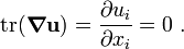
A resonant structure
Consider the periodic geometry shown in Figure 2. The matrix material has a high value of shear modulus () while the split-ring shaped region has a low shear modulus or is a void. The material inside the ring has the same shear modulus as the matrix material and is connected to the matrix by a thin ligament. The system is subjected to a
displacement in the direction (parallel to the axis of each
cylindrical split ring).
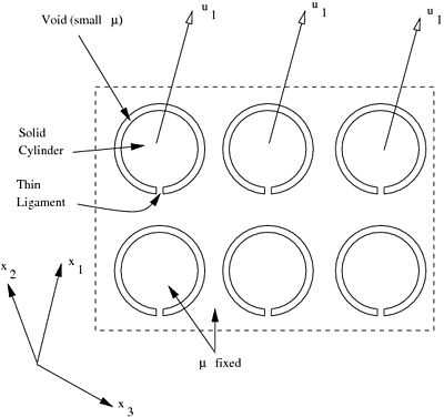 Figure 2. A periodic geometry containing split hollow cylinders of soft material in a matrix of stiff material. The direction is parallel to the axis of each cylinder. |
Clearly, each periodic component of the system behaves like a mass attached to a spring. This is a resonant structure and the effective density  can be negative. A detailed treatment of the problem can be found in Movchan04. Note that the governing equation for this problem is

Let us compare this problem with the TM case where  is the out of
plane magnetic induction. The governing equation now is
is the out of
plane magnetic induction. The governing equation now is
If the value of  in the region of the void (ring) is small and hence is large (which implies that the conductivity
  is large), analogy with the equation of elastodynamics implies that the effective permeability
  can be negative for this material.
References
- R. J. Atkin and N. Fox. An introduction to the theory of elasticity. Longman, New York, 1980.
- A. B. Movchan and S. Guenneau. Split-ring resonators and localized modes. Physical Review B, 70:125116, 2004.