Waves in composites and metamaterials/Anisotropic mass and generalization
< Waves in composites and metamaterialsThe content of these notes is based on the lectures by Prof. Graeme W. Milton (University of Utah) given in a course on metamaterials in Spring 2007.
Rigid Bar with Frequency Dependent Mass
Recall the a rigid bar with  cavities, each containing a spring-mass
system with mass
cavities, each containing a spring-mass
system with mass  and complex spring constant
  (see
Figure 1).
(see
Figure 1).
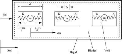 Figure 1. A rigid bar containing voids. Each void contains a spherical ball that is attached to the bar by springs. |
The momentum of the bar ( ) is related to its velocity (
 )
by the relation
)
by the relation
where  is the frequency and
  is the effective mass
which is given by
is the effective mass
which is given by
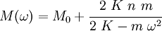
where  is the mass of the rigid bar~.
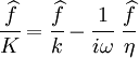
Let us now consider a specific model for the springs. A simple model
is the one-dimensional Maxwell model shown in Figure 2.
In this case instead of a spring with a complex spring constant we have
an elastic spring (with real spring constant  ) and a dashpot (with
a real viscosity
) and a dashpot (with
a real viscosity  ) in series. Let
  be the displacement of
the elastic spring and let
be the displacement of
the elastic spring and let  be that of the dashpot under the action of a
force
be that of the dashpot under the action of a
force  .
.
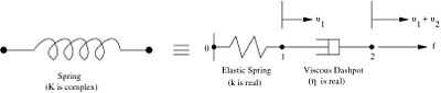 Figure 2. The Maxwell model for a spring with complex spring constant. |
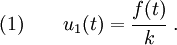
For the elastic spring, we have
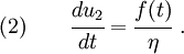
For the dashpot, we have
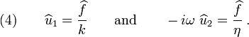
Once again, assuming that the functions  ,
,  , and
, and  can
be expressed as harmonic functions, we have
can
be expressed as harmonic functions, we have

Plugging equations (3) into equations (1) and (2), we get
Recall that the displacement  of the sphere of mass inside the cavity
is related to the applied force by the relation
of the sphere of mass inside the cavity
is related to the applied force by the relation
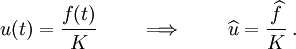
Now,  . Hence,
or,
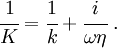
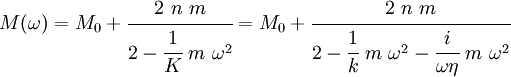
So, with the Maxwell model, the effective mass is
or,
This model is remarkably similar to a simple model for the frequency
dependent dielectric constant  .
.
Comparison with a simple model for
Consider the following simple model of an electron bound to an atom by a harmonic force under the influence of a slowly varying electric field (a detailed description can in found in Jackson75, Sec. 7.5). A schematic of the situation is shown in Figure 3.
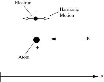 Figure 3. An electron bound by a harmonic force. |
Let the electric field be  and assume that it varies slowly in space
over the distance that the electron moves, i.e.,
and assume that it varies slowly in space
over the distance that the electron moves, i.e.,  . Let
be the mass of the electron
and let
. Let
be the mass of the electron
and let  be its charge. Let
  be the frequency of the
harmonic force binding the electron to the atom and let
be the frequency of the
harmonic force binding the electron to the atom and let  be a
damping coefficient due to interactions with obstacles.
be a
damping coefficient due to interactions with obstacles.
Then, the equation of motion of the electron is given by
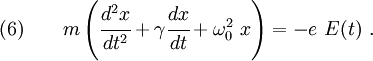
Let

Plugging equations (7) into equation (6), we get
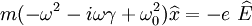
or
Let  be the charge density of the electron-atom system, i.e.,
![q(x,t) = -\delta[x(t)-x_0]~e + \delta(x_0-x_0)~e](../I/m/8d6d378c29bc807b58c2b0afba2ff71a.png)
where  is the Dirac delta function and
  is the position of the
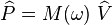
atom. Then, the dipole moment (the first moment of the charge) contributed by
the electron-atom system is given by
is the position of the
atom. Then, the dipole moment (the first moment of the charge) contributed by
the electron-atom system is given by
![p(t) = \int q(x,t)~x(t)~\text{d}x
= -e~\left[\int \delta[x(t)-x_0]~x(t)~\text{d}x +
\int \delta(0)~x(t)~\text{d}x\right] ~.](../I/m/b8828e1b2391cffa8ebc8fb0e9953ff2.png)
or,

Suppose now that instead of a binding frequency for all the
atoms and all the electrons in a volume, there are  atoms per unit volume
with binding
frequencies
atoms per unit volume
with binding
frequencies  and damping constants
  and. Then, we can
write the polarization as
and. Then, we can
write the polarization as
![\text{(8)} \qquad
\widehat{P} = \cfrac{e^2}{m} \left[\sum_i \cfrac{N_i}{
\omega_0^2 - \omega^2 - i\omega\gamma}\right]~\widehat{E}
= \left[\sum_i \cfrac{a_i}{\omega_0^2 - \omega^2 - i\omega\gamma}\right]
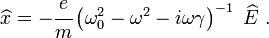
~\widehat{E}~.](../I/m/a3e7b141bbea787ec41e6590257ab23b.png)
Recall that the electric displacement is related to the electric field and the polarization by
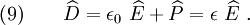
Therefore, from equations (8) and (9) we get
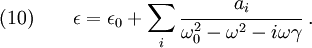
Comparing equation (5) with equation (10) we observe that they have the same form which implies that the effective permittivity is analogous to the effective mass. This also implies that the electric field is analogous to the velocity. Similarly, the polarization is analogous to the momentum.
More on frequency dependence of the mass
More generally, we get a frequency dependent density if all the constituents do not move in lock step. Lock step motion almost never occurs because there are thermal vibrations at the microscale. There are also many macroscopic situations in which lock step motion does not occur. Consider the example of a porous rock containing some water (see Figure 4). Both the rock grains and the water are connected, though this is not obvious from the figure
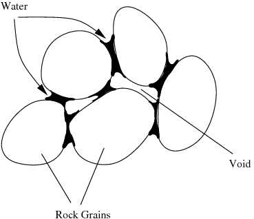 Figure 4. A porous rock containing some water. |
In this case, the water will move with a different frequency that the rock and the density of the composite will be dependent on the frequency.
At a molecular level, we can have a crystal with lead atoms attached by single bonds to the structure (see Figure 5). Presumably, the resonant frequency of such molecules is very high. so we will see the frequency dependence of the mass only at very high frequencies.
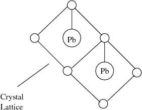 Figure 5. A crystal lattice containing lead atoms. |
In fact, Sheng et al. Sheng03 have shown in experiments that materials indeed have frequency dependent masses. An example of such a material is shown in Figure 6.
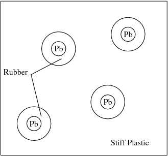 Figure 6. A composite material with frequency dependent mass. |
Generalizations of the Rigid Bar Model
Consider the rigid body containing cavities shown in Figure~7.
This is just a two-dimensional extension of the model shown in
Figure~1. Here and  are complex spring constants
in the
are complex spring constants
in the  and
and  directions.
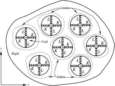 Figure 7. Schematic of a material with an anisotropic mass density. In this case the springs in each cavity are parallel to each other. |
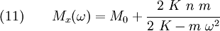
In this case, the effective mass along the -direction is given by
while that along the -direction is given by
In matrix form, we then have
 = M_0~\left[\mathsf{I}\right] + n~m~
\begin{bmatrix}
\cfrac{2~K}{2~K - m~\omega^2} & 0 \\
0 & \cfrac{2~L}{2~L - m~\omega^2}
\end{bmatrix} ~.
}](../I/m/2e4722cae9cd5e190025f29a0b2cc56e.png)
Hence, the effective mass is clearly anisotropic. Note however that from a macroscopic perspective it is not the average velocity in the matrix which is important. In fact, such a quantity does not even make sense because the velocity is not defined in the void phase. Rather it is the velocity of the matrix that is the relevant quantity in this model.
One can generalize the model one step further by having the springs be oriented at different angles to each other as shown in Figure 8. Also let the springs in each cavity have different spring constants and the masses in each cavity are different.
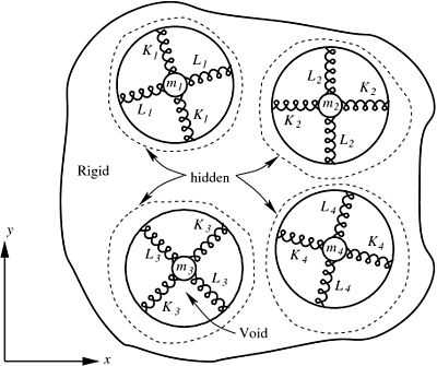 Figure 8. Schematic of a material in which the springs in each cavity are oriented at various angles to each other. |
In this case, let  be the rotation that is needed to orient each
set of springs with the and axes. Then, if
be the rotation that is needed to orient each
set of springs with the and axes. Then, if ![\left[\mathsf{R}\right]_j](../I/m/e6720ac148f5ffeb6d5cd6b3dc757fff.png) is the
rotation matrix for cavity
is the
rotation matrix for cavity  containing a mass
  , and if
  and
and  are the complex spring constants for that cavity, the effective
mass can be written as
are the complex spring constants for that cavity, the effective
mass can be written as
 = M_0~\left[\mathsf{I}\right] + \sum_{j=1}^n \left[\mathsf{R}\right]_j^T~
\begin{bmatrix}
\cfrac{2~K_j~m_j}{2~K_j - m_j~\omega^2} & 0 \\
0 & \cfrac{2~L_j~m_j}{2~L_j - m_j~\omega^2}
\end{bmatrix} \left[\mathsf{R}\right]_j ~.
}](../I/m/0b9b62970cdda8339f4efcd9ac074009.png)
The eigenvalues of  can therefore depend on .
General form of
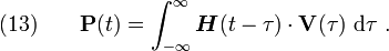
Take any body with a rigid matrix. Suppose, instead of applying harmonically
varying velocities, we apply a time varying velocity
 and observe what the momentum
  is. There will be some
linear constitutive relation
is. There will be some
linear constitutive relation
The kernel  is second-order tensor valued and may possibly
be singular. Also, since both
is second-order tensor valued and may possibly
be singular. Also, since both  and
and  are physical and real,
 must be real. Causality implies that
  when
when
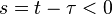 (or
(or  ) since the inertial force cannot depend
on velocities in the future.
) since the inertial force cannot depend
on velocities in the future.
Taking the Fourier transform of equation (13) and using the convolution theorem, we get

where
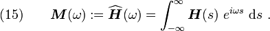
The quantity can be shown to satisfy the Cauchy-Riemann
equations only if  . This is a consequence of causality
 and the fact that the integral in equation (15) only
converges in the upper half of the complex plane.
\footnote{ Note the positive sign in
the power of
and the fact that the integral in equation (15) only
converges in the upper half of the complex plane.
\footnote{ Note the positive sign in
the power of  in equation (15). This occurs because
we have chosen the inverse Fourier transform to be of the form
in equation (15). This occurs because
we have chosen the inverse Fourier transform to be of the form
The effect of such a choice is that the imaginary part of is
positive instead of negative.} Hence, is analytic in
when . The quantity  is real.
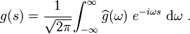
Now, the complex conjugate of is given by
where  denotes the complex conjugate of
  (for any complex
).
(for any complex
).
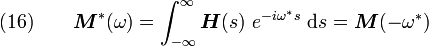
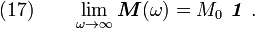
Also assume that, for large enough frequencies, the dynamic mass tends toward the static mass, i.e.,
Equation (15) can be used to establish the Kramers-Kronig
equations for the material. To do that,
recall Cauchy's formula for a function which is analytic on a domain
that is enclosed in a piecewise smooth curve  :
:
Since the function is analytic on the upper-half plane,
for any point in a closed contour in the upper-half plane, we
have
Let us now choose the contour such that it consists of the real
axis and a great semicircle at infinity in the upper half plane (see
Figure~9).
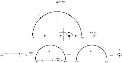 Figure 9. The closed curve that is used to evaluate the integral in equation (18). |
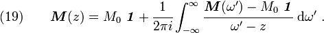
Also, from equation (17) we observe that

Hence, there is no contribution to the integral in equation (18) due to the semicircular part of the contour and we just have to perform an integration only over the real line:
Now, let us consider the integral
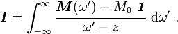
There is a pole at the point  (in the figure, the contour is
shown as a semicircle of radius
(in the figure, the contour is
shown as a semicircle of radius  centered at the pole). In the
limit
centered at the pole). In the
limit  , this integral may be interpreted to mean the
Cauchy principal value (not the same as principal values in complex analysis)
, this integral may be interpreted to mean the
Cauchy principal value (not the same as principal values in complex analysis)

From Figure~9 we observe that this integral can be
broken up into the integral over the path  minus the sum of the
integrals over the paths
minus the sum of the
integrals over the paths  and
and  . From the Cauchy-Goursat theorem,
the integral over the closed path is zero. We have also seen that
since
. From the Cauchy-Goursat theorem,
the integral over the closed path is zero. We have also seen that
since 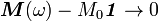 as
as  ,
the integral over is zero. The integral over the path around the
pole is obtained from the Residue Theorem (where the value is divided
by two because the integral is over a semicircle), i.e.,
,
the integral over is zero. The integral over the path around the
pole is obtained from the Residue Theorem (where the value is divided
by two because the integral is over a semicircle), i.e.,
![\oint_{D}
\cfrac{\boldsymbol{M}(\omega') - M_0~\boldsymbol{\mathit{1}}}{\omega' - z}~\text{d}\omega' =
-\pi i~[\boldsymbol{M}(z) - M_0\boldsymbol{\mathit{1}}] ~.](../I/m/9bbbee1e3c96aac92143aa0762a6e1e2.png)
The negative sign arises because the curve is traversed in the counter-clockwise direction.
Therefore,
![\boldsymbol{I} = P \int_{-\infty}^{\infty} \cfrac{\boldsymbol{M}(\omega') - M_0~\boldsymbol{\mathit{1}}}{\omega' - z}~\text{d}\omega'
= \pi i~[\boldsymbol{M}(z) - M_0\boldsymbol{\mathit{1}}] ~.](../I/m/470a68f9ea4b083cace08919cee35a65.png)
or,
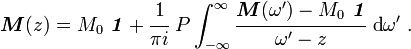
Letting  and taking the limit as , we
get
and taking the limit as , we
get
Note that, in the above equation, both and  are real.
Expanding equation (20) into real and imaginary parts and
collecting terms, we get the first form of the Kramers-Kronig relations
are real.
Expanding equation (20) into real and imaginary parts and
collecting terms, we get the first form of the Kramers-Kronig relations
![\text{(21)} \qquad
{
\begin{align}
\text{Re}[\boldsymbol{M}(\omega)] & = M_0~\boldsymbol{\mathit{1}} + \cfrac{1}{\pi}~
P \int_{-\infty}^{\infty} \cfrac{\text{Im}[\boldsymbol{M}(\omega')]}{\omega' - \omega}~\text{d}\omega' \\
\text{Im}[\boldsymbol{M}(\omega)] & = - \cfrac{1}{\pi}~
P \int_{-\infty}^{\infty} \cfrac{\text{Re}[\boldsymbol{M}(\omega')] - M_0~\boldsymbol{\mathit{1}}}
{\omega' - \omega}~\text{d}\omega' ~.
\end{align}
}](../I/m/7be1568d996f080552ddb7e05321922b.png)
Therefore, the real part of the frequency dependent mass can be determined if we know the imaginary part and vice versa.
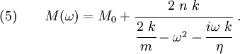
We can also eliminate the negative frequencies from equations (21). Recall from equation (16) that
Since, in equations (21), and are real, we have
This implies that
![\text{Re}[\boldsymbol{M}(\omega)] = \text{Re}[\boldsymbol{M}(-\omega)]
\qquad \text{and} \qquad
\text{Im}[\boldsymbol{M}(\omega)] = -\text{Im}[\boldsymbol{M}(-\omega)] ~.](../I/m/604e80c59bef9a210f009576704fb09a.png)
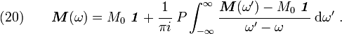
Consider the first of equations (21). We can write this relation as
![\begin{align}
\text{Re}[\boldsymbol{M}(\omega)] & = M_0~\boldsymbol{\mathit{1}} + \cfrac{1}{\pi}~\left\{
P \int_{-\infty}^{0} \cfrac{\text{Im}[\boldsymbol{M}(\omega')]}{\omega' - \omega}~\text{d}\omega' +
P \int_0^{\infty} \cfrac{\text{Im}[\boldsymbol{M}(\omega')]}{\omega' - \omega}~\text{d}\omega'
\right\}\\
& = M_0~\boldsymbol{\mathit{1}} + \cfrac{1}{\pi}~\left\{
P \int_0^{\infty} \cfrac{\text{Im}[\boldsymbol{M}(-\omega')]}{-\omega' - \omega}~\text{d}\omega' +
P \int_0^{\infty} \cfrac{\text{Im}[\boldsymbol{M}(\omega')]}{\omega' - \omega}~\text{d}\omega'
\right\}\\
& = M_0~\boldsymbol{\mathit{1}} + \cfrac{1}{\pi}~\left\{
-P \int_0^{\infty} \cfrac{-\text{Im}[\boldsymbol{M}(\omega')]}{\omega' + \omega}~\text{d}\omega' +
P \int_0^{\infty} \cfrac{\text{Im}[\boldsymbol{M}(\omega')]}{\omega' - \omega}~\text{d}\omega'
\right\}\\
& = M_0~\boldsymbol{\mathit{1}} + \cfrac{1}{\pi}~
P \int_0^{\infty} \text{Im}[\boldsymbol{M}(\omega')]\left[\cfrac{1}{\omega' + \omega}+
\cfrac{1}{\omega'-\omega}\right]~\text{d}\omega' \\
& = M_0~\boldsymbol{\mathit{1}} + \cfrac{2}{\pi}~
P \int_0^{\infty} \cfrac{\omega'~\text{Im}[\boldsymbol{M}(\omega')]}{\omega'^2 - \omega^2}
~\text{d}\omega' ~.
\end{align}](../I/m/a899d05c340be2116274e74ff11f83c5.png)
Similarly, the second of equations (21) may be written as
![\begin{align}
\text{Im}[\boldsymbol{M}(\omega)] & = - \cfrac{1}{\pi}~\left\{
P \int_{-\infty}^{0} \cfrac{\text{Re}[\boldsymbol{M}(\omega')] - M_0~\boldsymbol{\mathit{1}}}
{\omega' - \omega}~\text{d}\omega' +
P \int_0^{\infty} \cfrac{\text{Re}[\boldsymbol{M}(\omega')] - M_0~\boldsymbol{\mathit{1}}}
{\omega' - \omega}~\text{d}\omega' \right\} \\
& = - \cfrac{1}{\pi}~\left\{
-P \int_0^{\infty} \cfrac{\text{Re}[\boldsymbol{M}(-\omega')] - M_0~\boldsymbol{\mathit{1}}}
{\omega' + \omega}~\text{d}\omega' +
P \int_0^{\infty} \cfrac{\text{Re}[\boldsymbol{M}(\omega')] - M_0~\boldsymbol{\mathit{1}}}
{\omega' - \omega}~\text{d}\omega' \right\} \\
& = - \cfrac{1}{\pi}~\left\{
P \int_0^{\infty} (\text{Re}[\boldsymbol{M}(-\omega')] - M_0~\boldsymbol{\mathit{1}})\left[
-\cfrac{1}{\omega' + \omega} + \cfrac{1}
{\omega' - \omega}\right]~\text{d}\omega' \right\} \\
& = - \cfrac{2~\omega}{\pi}~\left\{
P \int_0^{\infty} \cfrac{\text{Re}[\boldsymbol{M}(-\omega')] - M_0~\boldsymbol{\mathit{1}}}
{\omega'^2 - \omega^2}~\text{d}\omega' \right\} ~.
\end{align}](../I/m/26e81a8254b0d53a6731042040528329.png)
Therefore, the alternative form of the Kramers-Kronig relations is
![\text{(22)} \qquad
{
\begin{align}
\text{Re}[\boldsymbol{M}(\omega)] & = M_0~\boldsymbol{\mathit{1}} + \cfrac{2}{\pi}~
P \int_0^{\infty} \cfrac{\omega'~\text{Im}[\boldsymbol{M}(\omega')]}{\omega'^2 - \omega^2}
~\text{d}\omega' \\
\text{Im}[\boldsymbol{M}(\omega)] & = - \cfrac{2~\omega}{\pi}~\left\{
P \int_0^{\infty} \cfrac{\text{Re}[\boldsymbol{M}(-\omega')] - M_0~\boldsymbol{\mathit{1}}}
{\omega'^2 - \omega^2}~\text{d}\omega' \right\} ~.
\end{align}
}](../I/m/e59de6c5cc58a227aa402413bd4dd1c5.png)
Significance of ![\text{Im}[\boldsymbol{M}(\omega)]](../I/m/3e5582221abf613193c9ee42113787fd.png)
Consider harmonically varying  and given by

Alternatively, we may write these as

Then,
which implies that
![\begin{align}
\text{Re}(\widehat{\mathbf{F}}) & = \omega~[\text{Re}(\boldsymbol{M})\cdot\text{Im}(\widehat{\mathbf{V}}) +
\text{Im}(\boldsymbol{M})\cdot\text{Re}(\widehat{\mathbf{V}})] \\
\text{Im}(\widehat{\mathbf{F}}) & = \omega~[\text{Im}(\boldsymbol{M})\cdot\text{Im}(\widehat{\mathbf{V}}) -
\text{Re}(\boldsymbol{M})\cdot\text{Re}(\widehat{\mathbf{V}})] ~.
\end{align}](../I/m/e06390a98da4b3f2c90ab94d8ce9cbfc.png)
The average rate of work done on the system in a cycle of oscillation will be
![\begin{align}
W & = \cfrac{\omega}{2~\pi}
\int_{0}^{2\pi/\omega}~\mathbf{F}(t)\cdot\mathbf{V}(t)~\text{d}t \\
& = \cfrac{\text{Re}(\widehat{\mathbf{F}})\cdot\text{Re}(\widehat{\mathbf{V}}) +
\text{Im}(\widehat{\mathbf{F}})\cdot\text{Im}(\widehat{\mathbf{V}})}{2} \\
& = \omega~[\text{Re}(\widehat{\mathbf{V}})\cdot\text{Im}[\boldsymbol{M}(\omega)]\cdot\text{Re}(\widehat{\mathbf{V}}) +
\text{Im}(\widehat{\mathbf{V}})\cdot\text{Im}[\boldsymbol{M}(\omega)]\cdot\text{Im}(\widehat{\mathbf{V}})].
\end{align}](../I/m/90b13d00531094090ebad3d4ebb18f27.png)
This quadratic form will be non-negative for all choices of  if
and only if
if
and only if  is positive semidefinite for all real
 . Note that the quadratic form does not contain
  .
Since the work done in a cycle should be zero in the absence of
dissipation, this implies that the imaginary part of the mass is
connected to the energy dissipation (for instance, into heat).
.
Since the work done in a cycle should be zero in the absence of
dissipation, this implies that the imaginary part of the mass is
connected to the energy dissipation (for instance, into heat).
References
J. D. Jackson. Classical Electrodynamics: 2nd Edition. John Wiley and Sons, New York, 1975.
P. Sheng, X. X. Zhang, Z. Liu, and C. T. Chan. Locally resonant sonic materials. Physica B. Condensed Matter, 338:201--205, 2003.