Physics/Essays/Fedosin/Velocity circulation quantum
< Physics < Essays < FedosinA velocity circulation quantum (VCQ), or quantum vortex, is an auxiliary physical quantity which can be used to calculate fictitious magnetic charge and fictitious torsion mass, as well as the magnetic flux quantum and strong gravitational torsion flux quantum. The value of the quantum vortex depends on the matter level according to Infinite Hierarchical Nesting of Matter.
Definition
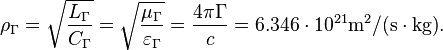
The velocity circulation quantum is calculated by the formula:
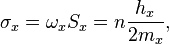
where  is the angular frequency of oscillation in system,
 is the effective surface area,
 is the quantum number which can be integer or fractional in the general case,
 is an action constant of the matter level,
 is a mass quantum of the matter level.
There are not very successful attempts to link with definite scale (Planck scale, Stoney scale, Natural scale, etc).
History
The first VCQ was proposed in the early 50-th for the quantum superfluids in the general form by R. Feynman [1]
and Abrikosov [2]
in the form of circulation of velocity  along the closed loop: [3]
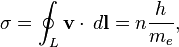
where  is the Planck constant as the action constant at the atomic level of matter,
  is the electron mass.
If  then circulation of velocity is:

The further developments of this approach was made by Yakymakha (1994) for inversion layers in MOSFETs . [4]
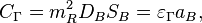
The velocity circulation quantum is important in gravitational model of strong interaction by Fedosin, in which  is proportional to strong gravitational torsion flux quantum. In particular nucleons equilibrium in nucleus depends on the equilibrium of strong gravitation attraction forces between nucleons and repulsive forces due to repulsion of the nucleons torsion fluxes. [5]
[6]
is proportional to strong gravitational torsion flux quantum. In particular nucleons equilibrium in nucleus depends on the equilibrium of strong gravitation attraction forces between nucleons and repulsive forces due to repulsion of the nucleons torsion fluxes. [5]
[6]
Electron quantum systems
Phase shifts
In the gravitational field with the 4-potential  and in electromagnetic field with the 4-potential
  the electron acquires phase shifts according to formulas: [7]

where  is the displacement 4-vector,
  is the elementary charge,
  is the Dirac constant.
The phase shift, obtained due to the electromagnetic 4-potential 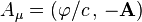 , is proved by the Aharonov-Bohm effect, when electric scalar potential
  , electric field strength
  and magnetic field
  are equal to zero, and there is only vector potential
  in the system. In the case with vector potentials of gravitational
  and electromagnetic fields phase shifts are:
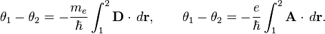
Since the gravitational torsion field  and the magnetic field
  then using Stokes' theorem we have:
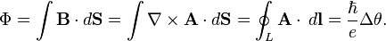
If circulation of electromagnetic vector potential results in change of phase  then magnetic flux is:
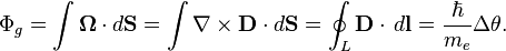
  . The same for gravitational vector potential and gravitational torsion flux gives:
  .
.
In superconductivity the electrons form pairs with the charge of a pair  so magnetic flux in the superconducting loop or a hole in a bulk superconductor is quantized. The single magnetic flux quantum in the case is
 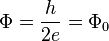 . Using of gravitational vector potential instead of electromagnetic vector potential in experiments gives single gravitational torsion flux quantum
  for electron superconductivity.
Bohr atom simple model
The Bohr radius is the averaged electron radius for the first energy level  :
:

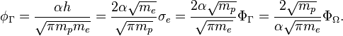
where  is the fine structure constant,
  is the Compton wavelength of electron,
and
is the Compton wavelength of electron,
and  is the speed of light.
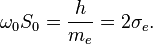
The angular frequency of electron rotation in atom is:

The flat surface area is:

Bohr velocity circulation quantum is:
The electron magnetic flux for the first energy level is:
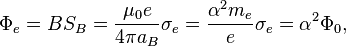
where  is the magnetic field in electron disc,
 is the vacuum permeability.
The strong gravitational electron torsion flux for the first energy level is:

where  is the gravitational torsion field of strong gravitation in electron disc,
 is the gravitomagnetic gravitational constant of selfconsistent gravitational constants in the field of strong gravitation,
 is the strong gravitational constant,
 is the vacuum permittivity,
 is the strong gravitational torsion flux quantum, which is related to proton with its mass
  .
.
Inversion layer "flat atom"
In experiments with inversion layers in MOSFETs there were found: [4]
Inversion layer surface area is:
 m2.
m2.
Inversion layer resonance frequency is:
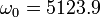 rad/s.
Resonator electromagnetic reactive parameters are:
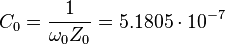 F,
F,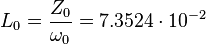 H,
H,
where 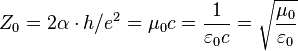 is the impedance of free space.
Yakymakha velocity circulation quantum is:
Bohr atom as a quantum resonator
Electromagnetic quantum resonator
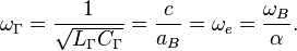
For the electromagnetic wave which runs in a circle with the Bohr radius in the electron matter the lowest resonance frequency is:
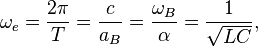
where  is the wave period,
  is the Bohr atom electric quantum inductance,
  is the Bohr atom electric quantum capacitance.
We can suppose that the wave impedance equals to impedance of free space:
With regard to these two equations the inductance and capacitance are as follows:
On the other hand in Bohr atom the electron in the form of a flat disc has density of states, the inductance and capacitance according to definition: [8]

From these equations the induced magnetic flux  and the induced charge
  can be found:

As it can be seen the induced magnetic flux related to the velocity circulation quantum  of the electron disc and exceed the electron magnetic flux
  of Bohr atom.
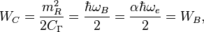
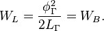
For the quantum electromagnetic resonator approach we can derive the following maximal values for the energies stored on capacitance and inductance:
The energy looks like the energy of quantum oscillator in zero state with the frequency  . But the real wave frequency is
  . So the action constant for the matter inside the electron with such wave is
  . The same follows from the Infinite Hierarchical Nesting of Matter where different action constants connected to different matter levels.
Gravitational quantum resonator
The gravitational quantum capacitance for Bohr atom is:
where 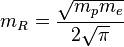 is the induced mass,
 is the gravitoelectric gravitational constant of selfconsistent gravitational constants in the field of strong gravitation.
The gravitational quantum inductance is:
where the induced gravitational torsion flux is:
The gravitational wave impedance is:
The resonance frequency of gravitational oscillation is:
For the quantum gravitational resonator approach we can derive the following maximal values for the energies stored on capacitance and inductance:
The energy  of the wave of strong gravitation in the electron matter has the same value as in case of rotating electromagnetic wave, and can be associated with the mass:
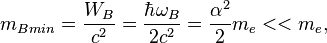
which could be named as the minimal mass-energy of the quantum resonator.
One way to explain the minimal mass-energy  is the supposition that Planck constant can be used at all matter levels including the level of star. As a result of the approach one should introduce different scales such as Planck scale, Stoney scale, Natural scale, with the proper masses and lengths. But such proper masses do not relate with the real particles.
Another way recognizes the similarity of matter levels and SPФ symmetry as the principles of matter structure where the action constants depend on the matter levels. For example there is the stellar Planck constant at the star level that describes star systems without any auxiliary mass and scales.
Applications for cosmic objects
Neutron star
The stellar Planck constant 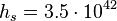 J• s can be found with the help of Planck constant and coefficients of similarity on mass, speed and size :

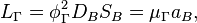
For the star with mass  of Solar mass the stellar gravitational torsion flux quantum is:
 m2/s.
m2/s.
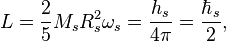
As in the case with the proton we should expect that the angular momentum of typical neutron star of mass  and radius
  equals to:
where  is the typical angular frequency of star rotation, and
  is the stellar Dirac constant.
We find that the stellar velocity circulation quantum equals to the stellar gravitational torsion flux quantum of the neutron star:

where  is the equatorial rotation speed, and effective area of the star is close to the star section:
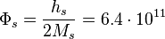
The gravitational torsion field in the center of star is: [6]
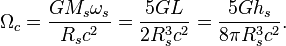
The product of  and the effective area of the star gives the stellar gravitational torsion flux of the star which is less then
  :
:
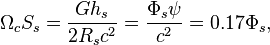
where  is the absolute value of scalar potential of gravitational field at the surface of the star,
  is the gravitational constant.
Solar system
For the velocity circulation quantum of a planet in the Solar system can be written:
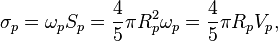
where  is the planet radius,
  is the equatorial rotation speed.
The planetary data are presented in the Table 1.
| Object | Radius, m | Equatorial rotation speed, m/s |  , m2/s , m2/s |
|---|---|---|---|
| Sun |  |
 |
 |
| Jupiter |  |
 |
 |
| Saturn |  |
 |
 |
| Neptun |  |
 |
 |
| Uran |  |
 |
 |
| Earth |  |
 |
 |
| Mars |  |
 |
 |
| Venus |  |
 |
 |
| Mercury |  |
 |
 |
By its meaning the velocity circulation quantum is proportional to angular momentum of body per unit of mass. We can see that the stellar gravitational torsion flux quantum is close to velocity circulation quanta of the Sun and big planets in the Solar system. With constant mass the gravitational torsion flux is conserved in the same degree as the angular momentum.
See also
References
- ↑ Feynman, R. P. (1955). Application of quantum mechanics to liquid helium. Progress in Low Temperature Physics 1: 17–53. ISSN 00796417.
- ↑ Abrikosov, A. A. (1957) "On the Magnetic properties of superconductors of the second group", Sov.Phys.JETP 5:1174-1182 and Zh.Eksp.Teor.Fiz.32:1442-1452.
- ↑ Putterman S.J. (1974). Superfluid hydrodynamics. North-Holland, Amsterdam.
- ↑ 4.0 4.1 Yakymakha O.L., Kalnibolotskij Y.M. (1994). "Very-low-frequency resonance of MOSFET amplifier parameters". Solid- State Electronics 37(10),1739-1751. Pdf
- ↑ Fedosin S.G. (1999), written at Perm, pages 544, Fizika i filosofiia podobiia ot preonov do metagalaktik, ISBN 5-8131-0012-1., http://lccn.loc.gov/2009457349
- ↑ 6.0 6.1 Sergey Fedosin, The physical theories and infinite hierarchical nesting of matter, Volume 1, LAP LAMBERT Academic Publishing, pages: 580, ISBN-13: 978-3-659-57301-9.
- ↑ Fedosin S.G. The Hamiltonian in Covariant Theory of Gravitation. Advances in Natural Science, 2012, Vol. 5, No. 4, P. 55 – 75.
- ↑ Serge Luryi (1988). "Quantum capacitance device". Appl.Phys.Lett. 52(6). Pdf