Vector calculus

Coordinate systems
Vectors
Coulomb's Law
More math links

Material from Vectors was moved^[1] here.

Here we extend the concept of vector to that of the vector field. A familiar example of a vector field is wind velocity: It has direction and magnitude, which makes it a vector. But it also depends on position (and ultimately on time). Wind velocity is a function of (x,y,z) at any given time, equivalently we can say that wind velocity is a time-dependent field: 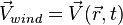$\vec V_{wind}=\vec V(\vec r, t)$ .

Derivative of a vector valued function

Let $\mathbf{a}(x)\,$ be a vector function that can be represented as

\mathbf{a}(x) = a_1(x) \mathbf{e}_1 + a_2(x) \mathbf{e}_2 + a_3(x) \mathbf{e}_3\,

where $x\,$ is a scalar.

Then the derivative of $\mathbf{a}(x)\,$ with respect to $x\,$ is

\cfrac{d\mathbf{a}(x)}{dx} = \lim_{\Delta x\rightarrow 0} \cfrac{\mathbf{a}(x+\Delta x) - \mathbf{a}(x)}{\Delta x} = \cfrac{da_1(x)}{dx} \mathbf{e}_1 + \cfrac{da_2(x)}{dx} \mathbf{e}_2 + \cfrac{da_3(x)}{dx} \mathbf{e}_3~.

Note: In the above equation, the unit vectors $\mathbf{e}_i$ (i=1,2,3) are assumed constant.
If $\mathbf{a}(x)\,$ and $\mathbf{b}(x)\,$ are two vector functions, then from the chain rule we get

\begin{align} \cfrac{d({\mathbf{a}}\cdot{\mathbf{b}})}{x} & = {\mathbf{a}}\cdot{\cfrac{d\mathbf{b}}{dx}} + {\cfrac{d\mathbf{a}}{dx}}\cdot{\mathbf{b}} \\ \cfrac{d({\mathbf{a}}\times{\mathbf{b}})}{dx} & = {\mathbf{a}}\times{\cfrac{d\mathbf{b}}{dx}} + {\cfrac{d\mathbf{a}}{dx}}\times{\mathbf{b}} \\ \cfrac{d[{\mathbf{a}}\cdot{({\mathbf{a}}\times{\mathbf{b}})}]}{dt} & = {\cfrac{d\mathbf{a}}{dt}}\cdot{({\mathbf{b}}\times{\mathbf{c}})} + {\mathbf{a}}\cdot{\left({\cfrac{d\mathbf{b}}{dt}}\times{\mathbf{c}}\right)} + {\mathbf{a}}\cdot{\left({\mathbf{b}}\times{\cfrac{d\mathbf{c}}{dt}}\right)} \end{align}

Scalar and vector fields

Let $\mathbf{x}\,$ be the position vector of any point in space. Suppose that there is a scalar function ( $g\,$ ) that assigns a value to each point in space. Then

g = g(\mathbf{x})\,

represents a scalar field. An example of a scalar field is the temperature. See Figure4(a).

Figure 4: Scalar and vector fields.

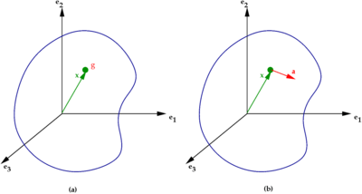
If there is a vector function ( $\mathbf{a}\,$ ) that assigns a vector to each point in space, then

\mathbf{a} = \mathbf{a}(\mathbf{x})\,

represents a vector field. An example is the displacement field. See Figure 4(b).

Gradient of a scalar field

Let $\varphi(\mathbf{x})\,$ be a scalar function. Assume that the partial derivatives of the function are continuous in some region of space. If the point $\mathbf{x}\,$ has coordinates ( $x_1, x_2, x_3\,$ ) with respect to the basis ( $\mathbf{e}_1, \mathbf{e}_2, \mathbf{e}_3\,$ ), the gradient of $\varphi\,$ is defined as

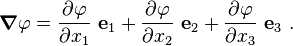
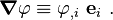
\boldsymbol{\nabla}{\varphi} = \frac{\partial \varphi}{\partial x_1}~\mathbf{e}_1 + \frac{\partial \varphi}{\partial x_2}~\mathbf{e}_2 + \frac{\partial \varphi}{\partial x_3}~\mathbf{e}_3 ~.

In index notation,

\boldsymbol{\nabla}{\varphi} \equiv \varphi_{,i}~\mathbf{e}_i ~.

The gradient is obviously a vector and has a direction. We can think of the gradient at a point being the vector perpendicular to the level contour at that point.

It is often useful to think of the symbol $\boldsymbol{\nabla}{}$ as an operator of the form

\boldsymbol{\nabla}{} = \frac{\partial }{\partial x_1} ~\mathbf{e}_1 + \frac{\partial }{\partial x_2} ~\mathbf{e}_2 + \frac{\partial }{\partial x_3} ~\mathbf{e}_3 ~.

Divergence of a vector field

If we form a scalar product of a vector field $\mathbf{u}(\mathbf{x})\,$ with the $\boldsymbol{\nabla}{}$ operator, we get a scalar quantity called the divergence of the vector field. Thus,

\boldsymbol{\nabla}\cdot\mathbf{u} = \frac{\partial u_1}{\partial x_1} + \frac{\partial u_2}{\partial x_2} + \frac{\partial u_3}{\partial x_3} ~.

In index notation,

\boldsymbol{\nabla}\mathbf{u} \equiv u_{i,i} ~.

If $\boldsymbol{\nabla}\mathbf{u} = 0$ , then $\mathbf{u}\,$ is called a divergence-free field.

The physical significance of the divergence of a vector field is the rate at which some density exits a given region of space. In the absence of the creation or destruction of matter, the density within a region of space can change only by having it flow into or out of the region.

Curl of a vector field

The curl of a vector field $\mathbf{u}(\mathbf{x})\,$ is a vector defined as

\boldsymbol{\nabla}\times{\mathbf{u}} = \det \begin{vmatrix} \mathbf{e}_1 & \mathbf{e}_2 & \mathbf{e}_3 \\ \frac{\partial }{\partial x_1} & \frac{\partial }{\partial x_2} & \frac{\partial }{\partial x_3} \\ u_1 & u_2 & u_3 \\ \end{vmatrix}

The physical significance of the curl of a vector field is the amount of rotation or angular momentum of the contents of a region of space.

Laplacian of a scalar or vector field

The Laplacian of a scalar field $\varphi(\mathbf{x})\,$ is a scalar defined as

\nabla^2{\varphi} := \boldsymbol{\nabla}(\boldsymbol{\nabla}{\varphi}) = \frac{\partial^2 \varphi}{\partial x_1} + \frac{\partial^2 \varphi}{\partial x_2} + \frac{\partial^2 \varphi}{\partial x_3}~.

The Laplacian of a vector field $\mathbf{u}(\mathbf{x})\,$ is a vector defined as

\nabla^2{\mathbf{u}} := (\nabla^2{u_1}) \mathbf{e}_1 + (\nabla^2{u_2}) \mathbf{e}_2 + (\nabla^2{u_3}) \mathbf{e}_3 ~.

Identities in vector calculus

Some frequently used identities from vector calculus are listed below.

$\boldsymbol{\nabla}(\mathbf{a} + \mathbf{b}) = \boldsymbol{\nabla}\cdot{\mathbf{a}} + \boldsymbol{\nabla}\cdot{\mathbf{b}}$
$\boldsymbol{\nabla}\times{(\mathbf{a} + \mathbf{b})} = \boldsymbol{\nabla}\times{\mathbf{a}} + \boldsymbol{\nabla}\times{\mathbf{b}}$
$\boldsymbol{\nabla}(\varphi\mathbf{a}) = \cdot{(\boldsymbol{\nabla}{\varphi})}{\mathbf{a}} + \varphi (\boldsymbol{\nabla}\cdot{\mathbf{a}})$
$\boldsymbol{\nabla}\times{(\varphi\mathbf{a})} = {(\boldsymbol{\nabla}{\varphi})}\times{\mathbf{a}} + \varphi (\boldsymbol{\nabla}\times{\mathbf{a}})$
$\boldsymbol{\nabla}({\mathbf{a}}\times{\mathbf{b}}) = {\mathbf{b}}\cdot{(\boldsymbol{\nabla}\times{\mathbf{a}})} - {\mathbf{a}}\cdot{(\boldsymbol{\nabla}\times{\mathbf{b}})}$

Fundamental theorems of vector calculus

One version of the fundamental theorem of one-dimensional calculus is

\int_a^b f\,'(x)dx = f(b) - f(a)

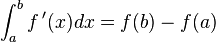
This is a theorem about a function, $f(x)$ , its first derivative, and a line segment. Two notations used to denote this line segment are [a,b] and the inequality, a<x<b. In the field of topology, $\partial$ denotes boundary. If we let the symbol $\mathcal L$ denote the infinite number of points in the line segment [a,b], then the symbol $\partial\mathcal L$ denotes the two endpoints (at x = a and x = b ) of the line segment $\mathcal L$ . These endpoints form the boundary of $\mathcal L$ .

Gradient theorem

The the gradient theorem is a direct generalization of the fundamental theorem of calculus:

\int_{\ell[\vec p \to \vec q] \subset \mathbb R^n} \vec\nabla f\cdot d\vec\ell = f \left(\vec{q}\right)- f\left(\vec{p}\right)

The subscript, $\ell[\vec p \to \vec q] \subset \mathbb R^n$ informs this is an integral over the over a one-dimensinal curve (or 'path') line integral $\ell$ from point $\vec r=\vec p$ to point $\vec r=\vec q$ . The function, $f= f(\vec r)$ is any scalar field that is differentiable. The expression $\subset \mathbb R^n$ informs us that $\vec r$ can be a member of an n-dimensional space. (In other words the theorem is easily generalized to more than three dimensions.) A consequence of this theorem is that 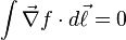$\int\vec\nabla f\cdot d\vec\ell=0$ for any "closed curve" The figure shows the closed curve A, as well as the "open curve", B. Two endpoints form the "boundary" of curve B.

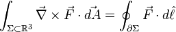
Stokes' theorem

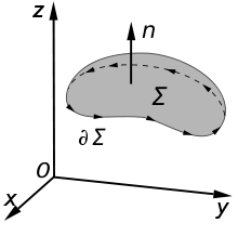
Stokes' theorem states:

\int_{\Sigma\subset\mathbb R^3} \vec\nabla \times \vec F \cdot \vec{dA} = \oint_{\partial\Sigma}\vec F\cdot d\hat\ell

The integral subscript, $\Sigma\subset \mathbb R^3$ informs us that this theorem is valid only in a three-dimensional vector space. The integral is over a two-dimensional surface,Σ ,with $\vec{dA} = \hat n dA$ , where $\hat n$ is normal to the surface. The integral over the surface, Σ, is nonzero only if its boundary, ∂Σ, exists. Surfaces with such boundaries are called open surfaces, and the boundary, ∂Σ, is a curve in 3-space that goes along the "edge" of the surface. This curve is integrated in the direction of positive orientation, meaning that $\vec{d\ell}$ and the surface normal follow $\hat n dA$ follow the right-hand rule.

Footnote: According to Wikipedia^[2], this form of the theorem was first discovered by Lord Kelvin, who communicated it to George Stokes in a letter dated July 2, 1850. Stokes set the theorem as a question on the 1854 Smith's Prize exam, which led to the result bearing his name.

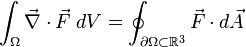
Divergence theorem

closed | open: Ω & ∂Ω

The divergence theorem states:

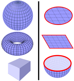
\int_{\Omega} \vec\nabla \cdot \vec F \;dV= \oint_{\partial \Omega\subset\mathbb R^3} \vec F \cdot d\vec A

The integral subscript, $\Omega\subset \mathbb R^n$ , informs us that this theorem is valid in an (arbitrary) n-dimensional vector space. The n-dimensional volume is Ω, and ∂Ω is its boundary. If n =3 dimensions, ∂Ω is a surface. Since this surface encloses a volume, it has no boundary of its own, and is therefore called a closed surface. The figure shows six surfaces. The three on the left have no boundary and are therefore closed; the ones to the right have a boundary (shown in red) and are therefore open. Note that the closed surfaces to the left are themselves boundaries volumes which are defined as what is "inside" the surface.

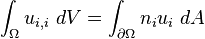
Footnote: In index notation, the gradient theorem can be written as

\int_{\Omega} u_{i,i}~dV = \int_{\partial\Omega} n_i u_i~dA

This article is issued from Wikiversity - version of the Sunday, June 22, 2014. The text is available under the Creative Commons Attribution/Share Alike but additional terms may apply for the media files.