Vectors

wikt:vector
w:Vector_(math...)
b:Vectors
w:Vector algebra relations
Coordinate systems*
Vector calculus*
Coulomb's Law*
More math links
* uses calculus

The basic idea

A vector is a mathematical concept that has both magnitude and direction. Detailed explanation of vectors may be found at Wikibooks linear algebra. In physics, vectors are used to describe things happening in space by giving a series of quantities which relate to the problem's coordinate system.

A vector is often expressed as a series of numbers. For example, in the two-dimensional space of real numbers, the notation (1, 1) represents a vector that is pointed 45 degrees from the x-axis towards the y-axis with a magnitude of $\sqrt 2$ .

Commonly in physics, we use position vectors to describe where something is in the space we are considering, or how its position is changing at that moment in time. Position vectors are written as summations of scalars multiplied by unit vectors. For example:

$\vec r= x \hat{i} + y \hat{j} + z \hat{k}$

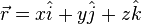
where x, y and z are scalars and $\hat{i}, \hat{j}$ and $\hat{k}$ are unit vectors of the Cartesian (René Descartes) coordinate system. A unit vector is a special vector which has magnitude 1 and points along one of the coordinate frame's axes. Unit vectors for each direction can be written as either $(\hat i,\hat j,\hat k)$ or $(\hat x,\hat y,\hat z)$ . The figure to the left illustrates this with $3\hat x + 2 \hat y$ . A vector itself is typically indicated by either an arrow: $\vec{v}$ , or just by boldface type: v, so the vector above as a complete equation would be denoted as:

$\vec{v} = v_x \hat{i} + v_y \hat{j} + v_z \hat{k}$

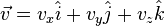
This velocity vector follows the convention that subscripts denote the components $(v_x, v_y, v_z)$ of the velocity vector. Writing the components of $\vec r$ as $(r_x, r_y, r_z)$ would be more consistent but is almost never done.

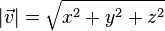
You can find the magnitude of a vector with this formula 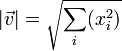$|\vec{v}| = \sqrt{\sum_i(x_i^2)}$ . For example, in two-dimensional space, this equation reduces to:

$|\vec{v}| = \sqrt{x^2+y^2}$ .

For three-dimensional space, this equation becomes:

$|\vec{v}| = \sqrt{x^2+y^2+z^2}$ .

Exercises

Find the magnitude of the following vectors.

$\vec{v} = (4, 3)$

$\vec{v} = (5, 3)$

$\vec{v} = (1, 0)$

click to view answers

$|\vec{v}| = 5$

$|\vec{v}| = \sqrt{34}$

$|\vec{v}| = 1$

Using vectors in physics

Many problems, particularly in mechanics, involve the use of two- or three-dimensional space to describe where objects are and what they are doing. Vectors can be used to condense this information into a precise and easily understandable form that is easy to manipulate with mathematics.

Position - or where something is, can be shown using a position vector. Position vectors measure how far something is from the origin of the reference frame and in what direction, and are usually, though not always, given the symbol $\vec{r}$ . It is usually good practice to use $\vec{r}$ for position vectors when describing your solution to a problem as most physicists use this notation.

Velocity is defined as the rate of change of position with respect to time. You may be used to writing velocity, v, as a scalar because it was assumed in your solution that v referred to speed in the direction of travel. However, if we take the strict definition and apply it to the position vector, which is usually written:

$\vec r =\vec r(t) = x\hat i + y\hat j + z\hat k$

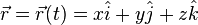
Taking the time derivative:

$\frac{d\vec{r}}{dt} = \frac{d}{dt}\left( x\hat i + y\hat j + z\hat k \right)= \frac{dx}{dt}\hat{i} + \frac{dy}{dt}\hat{j} + \frac{dz}{dt}\hat{k}$

We did not take the derivatives of the unit vectors because they are not changing. If the unit vectors are rotating, it is possible to take (vector) derivatives of them and derive the Coriolis force^[1]

Two types of vectors

Free vectors

Vectors that can be described by expressing their magnitude and direction.

Localized vectors

Vectors that cannot be described completely by just specifying its magnitude and direction, but also by specifying the line along which its representative segment lies. The tails of such vectors are always fixed.

Other types of basis vectors

Figure 1: A vector and its basis. b_j=a·g_j/g_j is the projection of a on g_j but is not a component if g_j are the basis vectors (j=1,2)

A vector is an object that has certain properties:

a vector has a magnitude (or length)
a vector has a direction.

To make the definition of the vector object more precise we may also say that vectors are objects that satisfy the properties of a vector space.

The standard notation for a vector is lower case bold type (for example $\mathbf{a}\,$ ).

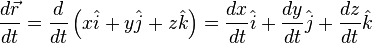
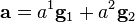
In Figure 1(a) you can see a vector $\mathbf{a}$ in red. This vector can be represented in component form with respect to the basis ( $\mathbf{e}_1, \mathbf{e}_2\,$ ) as

\mathbf{a} = a_1 \mathbf{e}_1 + a_2 \mathbf{e}_2 \,

where $\mathbf{e}_1\,$ and $\mathbf{e}_2\,$ are orthonormal unit vectors:

a_1= \mathbf{a}\cdot\mathbf{e}_1

and

a_2= \mathbf{a}\cdot\mathbf{e}_2

Recall that unit vectors are vectors of length 1. These vectors are also called basis vectors. In three or more dimensions an orthonormal basis we can write

\mathbf{a} = a_1 \mathbf{e}_1 + a_2 \mathbf{e}_2 + a_2 \mathbf{e}_3 \,

Basis vectors that are not orthonormal

You could also represent the same vector $\mathbf{a}\,$ in terms of another set of basis vectors ( $\mathbf{g}_1,\mathbf{g}_2\,$ ) as shown in Figure 1(b):

\mathbf{a} = a^1 \mathbf{g}_1 + a^2 \mathbf{g}_2 \,

In this space, the components of the vector are $(a^1,a^2)\,$ , which are not equal to the projections, $(b_1,b_2)\,$ that are shown in the figure. However as can be seen by inspecting the figure:

a^1\ne \mathbf{a}\cdot\mathbf{g}_1

and

a^2\ne \mathbf{a}\cdot\mathbf{g}_2

Click here to a non-orthonormal basis vectors in solid state physics

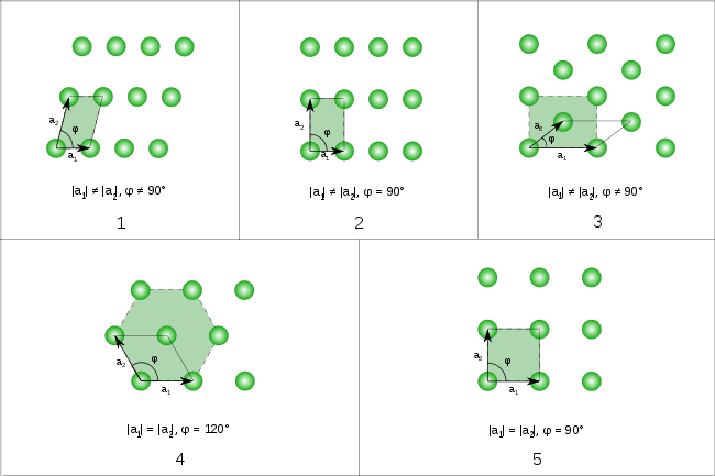
In solid state physics it is convenient for the basis vectors to represent displacements among nearest neighboring atoms. The basis vectors are neither normal nor orthogonal.

The five fundamental two-dimensional Bravais lattices: 1 oblique, 2 rectangular, 3 centered rectangular (rhombic), 4 hexagonal, and 5 square

Orthonormal basis vectors that are rotated

Another example of an alternative coordinate system is the rotated coordinate system:

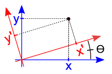
Click here for a derivation of the rotation matrix

Rotation of coordinates

From Wikipedia^[2], only a single angle is needed to specify a rotation in two dimensions – the angle of rotation, as defined in the figure. This figure depicts a passive (or alias) transformation in which the point remains stationary while the basis vectors are rotated.

While such transformations will not often be used, a deep understanding of them will yield insights relevant to relativity and quantum mechanics. It is important to know how this transformation can be derived as a matrix transformation. For that reason we will carefully derive how the primed and unprimed coordinates are related when:

\vec r = x\hat x + y\hat y = x'\hat x' + y'\hat y'

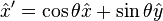
We begin by considering the active (or alibi) transformation of the unit vectors. Using well known and elementary properties concerning the components of a vector, we have:

\hat x' = \cos\theta\hat x + \sin\theta\hat y

\hat y' = -\sin\theta\hat x + \cos\theta\hat y

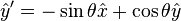
These two equations are valuable because they allow us to calculate dot products between the primed and unprimed basis vectors:

$\hat x'\cdot\hat x = \cos\theta\,\qquad\hat x'\cdot\hat y =\sin\theta\,\qquad\hat y'\cdot\hat x = -\sin\theta\,\qquad\hat y'\cdot\hat y =\cos\theta$

These dot products allow us to solve for any component of the primed or unprimed components of a vector. For example to find $x'$ we take the dot product with $\hat x'$ :

\hat x'\cdot\left(x'\hat x' + y'\hat y' \right)= \left(x\hat x + y\hat y\right)

simplifying, we have

x'(\hat x'\cdot\hat x') + y'(\hat x'\cdot\hat y' ) = x(\hat x'\cdot\hat x) + y(\hat x'\cdot\hat y)

and therefore,

x'=x\cos\theta +y\sin\theta

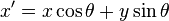This result can also be obtained without using unit vectors.^[3] Note how we used the dot product (also called inner product) to simplify the equations, using the property that the inner product between orthogonal vectors vanish. This concept can also be applied to infinite dimensional vector spaces, including functions, which under certain circumstances can be viewed as vectors. The results of such generalizations include Fourier transforms and the bra/ket notation of quantum mechanics.

Other permutations of this procedure yield two matrix equations:

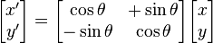$\begin{bmatrix} x' \\ y' \end{bmatrix} = \begin{bmatrix} \cos \theta & +\sin \theta \\ -\sin \theta & \cos \theta \end{bmatrix} \begin{bmatrix} x \\ y \end{bmatrix}$ and $\begin{bmatrix} x \\ y \end{bmatrix} = \begin{bmatrix} \cos \theta & -\sin \theta \\ +\sin \theta & \cos \theta \end{bmatrix} \begin{bmatrix} x' \\ y' \end{bmatrix}$ .

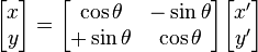Vector Algebra Operations

Figure 2: Vector operations.

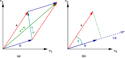
Addition and Subtraction

If $\mathbf{a}\,$ and $\mathbf{b}\,$ are vectors, then the sum $\mathbf{c} = \mathbf{a} + \mathbf{b}\,$ is also a vector (see Figure 2(a)).

The two vectors can also be subtracted from one another to give another vector $\mathbf{d} = \mathbf{a} - \mathbf{b}\,$ .

Multiplication by a scalar

Multiplication of a vector $\mathbf{b}\,$ by a scalar $\lambda\,$ has the effect of stretching or shrinking the vector (see Figure 2(b)).

You can form a unit vector ${\mathbf{\hat b}}\,$ that is parallel to $\mathbf{b}\,$ by dividing by the length of the vector $|\mathbf{b}|\,$ . Thus,

{\mathbf{\hat b}} = \cfrac{\mathbf{b}}{|\mathbf{b}|} ~.

Scalar product of two vectors

The scalar product or inner product or dot product of two vectors is defined as

\mathbf{a}\cdot\mathbf{b} = |\mathbf{a}||\mathbf{b}|\cos(\theta)

where $\theta\,$ is the angle between the two vectors (see Figure 2(b)).

If $\mathbf{a}\,$ and $\mathbf{b}\,$ are perpendicular to each other, $\theta = \pi/2\,$ and $\cos(\theta) = 0\,$ . Therefore, ${\mathbf{a}}\cdot{\mathbf{b}} = 0$ .

The dot product therefore has the geometric interpretation as the length of the projection of $\mathbf{a}\,$ onto the unit vector $\hat{\mathbf{b}}\,$ when the two vectors are placed so that they start from the same point.

The scalar product leads to a scalar quantity and can also be written in component form (with respect to a given basis) as

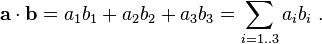
{\mathbf{a}}\cdot{\mathbf{b}} = a_1 b_1 + a_2 b_2 + a_3 b_3 = \sum_{i=1..3} a_i b_i~.

If the vector is $n$ dimensional, the dot product is written as

{\mathbf{a}}\cdot{\mathbf{b}} = \sum_{i=1..n} a_i b_i~.

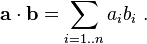
Using the Einstein summation convention, we can also write the scalar product as

{\mathbf{a}}\cdot{\mathbf{b}} = a_i b_i~.

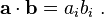
Also notice that the following also hold for the scalar product

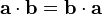${\mathbf{a}}\cdot{\mathbf{b}} = {\mathbf{b}}\cdot{\mathbf{a}}$ (commutative law).
${\mathbf{a}}\cdot{(\mathbf{b}+\mathbf{c})} = {\mathbf{a}}\cdot{\mathbf{b}} + {\mathbf{a}}\cdot{\mathbf{c}}$ (distributive law).

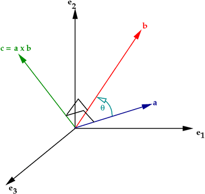
Vector product of two vectors

The vector product (or cross product) of two vectors $\mathbf{a}\,$ and $\mathbf{b}\,$ is another vector $\mathbf{c}\,$ defined as

\mathbf{c} = {\mathbf{a}}\times{\mathbf{b}} = |\mathbf{a}||\mathbf{b}|\sin(\theta) \hat{\mathbf{c}}

where $\theta\,$ is the angle between $\mathbf{a}\,$ and $\mathbf{b}\,$ , and $\hat{\mathbf{c}}\,$ is a unit vector perpendicular to the plane containing $\mathbf{a}\,$ and $\mathbf{b}\,$ in the right-handed sense (see Figure 3 for a geometric interpretation)

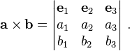
Figure 3: Vector product of two vectors.

In terms of the orthonormal basis $(\mathbf{e}_1,\mathbf{e}_2,\mathbf{e}_3)\,$ , the cross product can be written in the form of a determinant

{\mathbf{a}}\times{\mathbf{b}} = \begin{vmatrix} \mathbf{e}_1 & \mathbf{e}_2 & \mathbf{e}_3 \\ a_1 & a_2 & a_3 \\ b_1 & b_2 & b_3 \end{vmatrix}~.

In index notation, the cross product can be written as

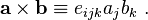
{\mathbf{a}}\times{\mathbf{b}} \equiv e_{ijk} a_j b_k ~.

where $e_{ijk}$ is the Levi-Civita symbol (also called the permutation symbol, alternating tensor).

Identities from Vector Algebra

Some useful vector identities are given below.

${\mathbf{a}}\times{\mathbf{b}} = - {\mathbf{b}}\times{\mathbf{a}}$
${\mathbf{a}}\times{\mathbf{b}+\mathbf{c}} = {\mathbf{a}}\times{\mathbf{b}} + {\mathbf{a}}\times{\mathbf{c}}$
${\mathbf{a}}\times{({\mathbf{b}}\times{\mathbf{c}})} = \mathbf{b}({\mathbf{a}}\cdot{\mathbf{c}}) - \mathbf{c}({\mathbf{a}}\cdot{\mathbf{b}})$
${({\mathbf{a}}\times{\mathbf{b}})}\times{\mathbf{c}} = \mathbf{b}({\mathbf{a}}\cdot{\mathbf{c}}) - \mathbf{a}({\mathbf{b}}\cdot{\mathbf{c}})~$
${\mathbf{a}}\times{\mathbf{a}} = \mathbf{0}~$
${\mathbf{a}}\cdot{({\mathbf{a}}\times{\mathbf{b}})} = {\mathbf{b}}\cdot{({\mathbf{a}}\times{\mathbf{b}})} = \mathbf{0}~$
${({\mathbf{a}}\times{\mathbf{b}})}\cdot{\mathbf{c}} = {\mathbf{a}}\cdot{({\mathbf{b}}\times{\mathbf{c}})}~$

The rest of this resource has been moved to Vector calculus.

The deleted material can be found at this permalink: https://en.wikiversity.org/w/index.php?title=Vectors&oldid=1194622

This article is issued from Wikiversity - version of the Wednesday, April 06, 2016. The text is available under the Creative Commons Attribution/Share Alike but additional terms may apply for the media files.