Statistical thermodynamics
Here we attempt to connect three iconic equations in thermodynamics: (1) the Clausius definition of entropy, (2) the Maxwell-Boltzmann energy distribution, and (3) the various statistical definitions of entropy. Of all the topics in the curriculum of the advanced physics major, thermodynamics is probably the subject presented with the most unanswered questions. To review what most students do learn:
- Thermometers don't work. A thermometer can only take its own temperature: Zeroth Law of Thermodynamics
- You can't win. Energy cannot be created: First Law of Thermodynancs
- You must lose. Friction is everywhere, friction turns to heat, and you can't use heat: Second Law of Thermodynamics
- It never ends.[1] The effort to reach absolute zero never succeeds: Third Law of Thermodynamics
- Nobody knows what entropy really is... vaguely attributed to John von Neumann.[2]
Three iconic equations in thermodynamics
Consider three iconic equations encountered in the education of a physicist:
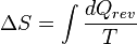
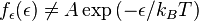
Thermodynamic entropy: In 1862 Clausius proposed that entropy is[3][4]
 (1)
(1)
where dQ is heat transferred during reversible heat flow (at constant volume). Heat is energy that spontaneously flows when objects of different temperatures are placed in thermal contact.
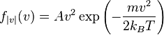
Maxwell-Boltzmann distribution for the ideal gas: In 1860 Maxwell produced a symmetry[5] argument that eventually led to a form of the Maxwell-Boltzmann distribution equation for of the speed (not velocity) of atoms in an ideal gas:
 (2)
(2)
where, 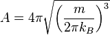 is a normalization constant, and kB (or k) is Boltzmann's constant, kB, equals 1.38062 x 10⁻²³ J/K.
Statistical definition of entropy:

(3) 
Our third equation, originally formulated by Ludwig Boltzmann between 1872 and 1875, is so iconic that it appears on Boltzmann's tombstone[6]. (using  instead of the modern
  for what is often called the 'number of available states')
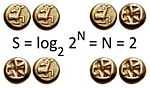
The existence of two definitions (k ln Ω and ʃdQ/T) for the same entity leaves one wondering if they are actually the same thing. Adding to the complexity is the fact that Ω in equation (3) has a number of definitions. For example, in information theory the constant, kB, equals one, and entropy is measured in 'bits' if the base of the logarithm is 2 (instead of base-e as used in physics). Information Ω is the inverse of probability if all probabilities are equal. And if all probabilities are equal, then Ω is the number of possible outcomes. The number of fair coin tosses is its entropy in bits. (Since there are 2N outcomes for N fair coins, and log2N2=N). In physics, entropy can be troublesome to calculate primarily due to issues concerning the appropriate number of equally probable states.[7] Another vexing problem is the fact that the equations of Newtonian and Hamiltonian physics possess time reversal symmetry, while reality apparently does not. Entropy reflects that reality by only increasing as time evolves.
for what is often called the 'number of available states')
The existence of two definitions (k ln Ω and ʃdQ/T) for the same entity leaves one wondering if they are actually the same thing. Adding to the complexity is the fact that Ω in equation (3) has a number of definitions. For example, in information theory the constant, kB, equals one, and entropy is measured in 'bits' if the base of the logarithm is 2 (instead of base-e as used in physics). Information Ω is the inverse of probability if all probabilities are equal. And if all probabilities are equal, then Ω is the number of possible outcomes. The number of fair coin tosses is its entropy in bits. (Since there are 2N outcomes for N fair coins, and log2N2=N). In physics, entropy can be troublesome to calculate primarily due to issues concerning the appropriate number of equally probable states.[7] Another vexing problem is the fact that the equations of Newtonian and Hamiltonian physics possess time reversal symmetry, while reality apparently does not. Entropy reflects that reality by only increasing as time evolves.
The goal of this essay is to connect equations (1), (2) and (3) by actual calculation.
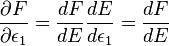
Thermodynamic (Clausius) definition of entropy
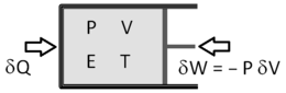
State variables: Pressure (P), Energy (E), Volume (V), and Temperature (T):
A state variable is a measurable physical property that can be uniquely defined for a substance that is in thermal, mechanical, and chemical equilibrium. We shall refer to this substance as 'the system' and two systems play a key role in this discussion:
- The monatomic ideal gas. The ideal gas model tends to fail at lower temperatures or higher pressures, when intermolecular forces and molecular size become important, and more complex ideal gasses, such as the diatomic molecule require quantum mechanics to understand rotational energy. These complications render such systems unsuitable to be fully modeled.
- At the opposite extreme, we are investigating any system (however complex) in what is called thermodynamic equilibrium. One requirement for being in thermodynamic equilibrium is that the pressure and temperature are both uniform throughout the system. Thermodynamics is often applied as an approximation when these conditions do not hold (for example when calculating the speed of sound).
Pressure and volume can be measured by observing the force and location of the piston, respectively. Temperature was originally measured with thermometers, but for our purposes the ideal gas thermometer is more convenient. We therefore establish the following operational definition of temperature:
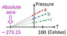
The temperature of a substance is such that when placed in a thermal contact with a monatomic heat bath,  where
where  is heat flow, and temperature is found by solving the equation of state for an ideal monatomic gas:
 (Equation of state for ideal gas)
Here, N is the number of particles (assumed constant in this introduction to classical thermodynamics), n is the number of moles, and R is called the gas constant. When classical thermodynamics was being constructed in the eighteenth and nineteenth centuries, it was not yet known that one mole consists of 6.022×10²³ atoms. Instead, the mole was defined as equal to the number of carbon atoms in 12 grams of carbon, and the gas constant, R, was an experimentally known parameter equal to 8.314 JK-1mol-1.
We shall assume that energy is a property of all systems of particles and that energy can be uniquely determined by other state variables. This brings our list of state variables to four:
- Volume (V)
- Pressure (P)
- Temperature (T)
- Energy(E)
Any function of these state variables is also a state variable. Generally speaking, any two state variables is sufficient to determine the system. One exception is energy for an ideal gas, where since energy is directly proportional to temperature, energy and temperature are insufficient for determining the state of an ideal gas.
Heat, work and the heat engine
Heat,, is the flow of energy from a hot to a cold substance. (The fact that heat never flows between objects with the same temperature is part of the zeroth law of thermodynamics.)
Work is  , where the minus sign ensures that dE, dW, and dQ are all positive if they add energy to the system. Since work and heat are the only two ways energy can enter or leave this sealed system, we have,
 First law with differentials; eventually becomes dE=TdS-PdV.
Why heat and work are not state variables
To understand why heat, , and work
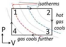
  are not state variables,we introduce the heat engine, which is a cycle that converts heat into work (or it can act as a heat pump if the cycle is reversed.) Since only two state variables are independent, it is possible to fully specify a system as a point on a two dimensional graph, for example on the P-V (pressure-volume) diagram shown in the figure. The other state variable (T) can be depicted using contours on the graph. Contours of constant temperature are called isotherms. For the ideal gas, these contours are hyperbolas, but we are not restricting our discussion to the ideal gas.
This figure shows pressure (P) as positive, but an equivalent P-V diagram could be constructed for an substance with negative pressure, such as a rubber band. The rubber band is a good example of approximate thermodynamic equilibrium because the system is never properly in chemical equilibrium - the cycles would not exactly close upon themselves as the rubber degrades into a more stable (but less desirable) substance. Nevertheless, one can construct a rubber band heat engine or heat pump: Stretch a thick rubberband and hold it stretched until it cools off to room temperature. Then decompress the rubberband and press it to your lips. It will feel cool because you have created a heat engine in reverse, called a heat pump (or a refrigeration unit).
Wikipedia refers to the cycle shown in the figure to the right as an Ideal Heat Engine. It is 'ideal' only in the sense that certain aspects are easy for students to calculate. From points 1-2, energy in the form of work leaves the system. No work is done from points 2-3 because the piston remains motionless. Work energy does re-enter the system from points 3-4, but less work is involved because the pressure is lower.
- The work done by the engine per cycle equals to the area enclosed by the cycle on a P-V diagram.
This equivalence of work performed to area inside the cycle on a P-V plot is a general property of heat engines.
By conservation of energy, the work performed by the engine must equal the energy that enters, and this energy can only be delivered into the system as heat. Since work energy leaves the engine at each cycle, and heat energy enters, work and heat are not state variables. It is meaningless to ask how much 'heat is in a system'. It is best to always write work and heat using notation that reflects this fact, e.g.,  and
and  .
.
How do we know that entropy even exists? The Clausius definition of entropy as the integral, dS =ʃdQ/T, defines entropy only as a differential. As we have seen, this does not prove that entropy is a state variable. The next section answers that question.
Carnot's Theorem
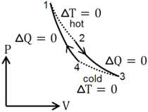
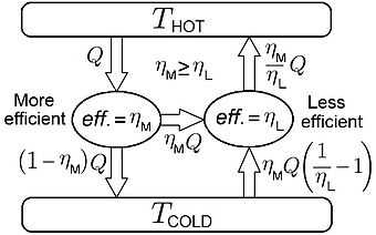
The 'ideal heat cycle' described above is easy to understand because work is so easy to calculate. Another heat engine is far more important. The Carnot cycle consists of four legs. Two legs are 'isotherms' with ΔT=0, (temperature remains constant), and two legs are 'adiabats' with ΔQ=0 (no heat flows). It can be shown that the Carnot cycle is the most efficient way to do work by transferring heat from a reservoir at Thot to a reservoir Tcold. But a far more important property of the Carnot cycle is the fact that all substances have exactly the same efficiency when used in a Carnot cycle. This can be proven using the diagram shown to the right. If two substances produced work with different efficiency, one could use the less efficient substance in a heat pump (i.e., air conditioner) and violate the second law of thermodynamics generating useful work from a temperature reservoir without the requirement that heat must be dumped into a colder reservoir. (As discussed below, this would permit the construction of a perpetual motion machine of the second kind.)
The efficiency of a heat engine operating between two temperatures is the ratio net work (per cycle) to the heat flow out of the hot reservoir (per cycle). Ideally, one would want to convert all the heat from the hot reservoir into work and not 'dump' any 'waste heat' into the cold reservoir. The proof that all Carnot cycles have the same efficiency can be found on this Wikipedia article.
Why the Carnot engine is reversible
Key to the proof is the fact that the second engine in the figure to the right is being operated in reverse as a [w: heat pump|] (refrigeration unit). Carnot's theorem does not hold if the engine is not reversible. The Carnot cycle shown in the figure to the left is reversible because heat enters at constant temperature. Strictly speaking, the Carnot cycle is only reversible if the temperature of the substance equals the temperature of the heat reservoir. It may seem odd that two systems (reservoir and substance inside the piston) are exchanging heat when both are at the same temperature, as heat only flows between bodies of unequal temperature. This paradox is resolved by admitting that the two temperatures are not exactly equal, but only approximately equal. And since a heat flow is often directly proportional to the difference in temperature, a true Carnot cycle would almost take an infinite amount of time to accomplish. The Carnot engine is truly an idealized and theoretical construct that can never truly exist. But something arbitrarily close to a Carnot engine can be built, and will operate in reverse in approximately the same fashion.
Why the Carnot engine is important
It is not uncommon for a heat engine to employ a complicated substance (e.g. Freon in an air conditioning unit). Carnot's theorem is a statement about all substances that remain in equilibrium throughout the cycle of a heat engine. If we can fully understand just one simple substance, then we can learn something that is true for all substances in equilibrium. The thing that we learn about will be called entropy. And the substance that we shall (attempt to) fully understand is the monatomic ideal gas.
- For an understanding of how the Carnot theorem establishes entropy as a state variable, see
An introduction to motion in phase space
Both the derivation of the Maxwell-Boltzmann equation for energy distribution, as well as the calculation of entropy in would today be called the spirit of information entropy require a deep understanding of how particles move in phase space. Phase space typically has twice the number of dimensions as the 'configuration space' students initially use to visualize motion. For example, instead of viewing motion in the two dimensional (x-y) plane, phase space would include four dimensions (x, y, vx, vy).
- For a deeper understanding of phase space, see:
Ergodic hypothesis and second law of thermodynamics

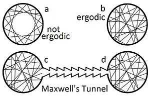
For simplicity we develop ideas with unphysical models. Consider a two dimensional gas of rays for which speed is irrelevant. They never collide, and change direction only after hitting a wall. If the walls are perfectly smooth, most particles would follow paths resembling that shown in (a) of the figure. Such an orbit does not occupy all of its available phase space, and is therefore called non-ergodic. Not only do these paths fail to fill the available phase space, they do not seem uniformly fill the space available to them. But if the smooth surfaces have any flaws, no matter how small, a gas of such particles would eventually fill the area uniformly, as shown in (b). In classical thermodynamics, the assumption is made that particles fill their available phase space uniformly in this fashion. This is called the ergodic hypothesis, and it was originally proposed by L. Boltzmann.[8]
Although we do not yet know why, it is clear that any trick to coax the gas from one of the two connected circles (c) and (d) using an artfully shapted tunnel as shown in the figure would fail. If such a tunnel ever managed to create a significant pressure difference, it could drive a perpetual motion machine of the second kind.[9] An automobile's pistons would be driven by arranging for the atoms to randomly find their way to one side of a piston. The compressed air would expand to power the car. In expanding in this fashion the air would cool. But the exhaust from this engine would be cold air, some of which could be pumped directly into the cab on a hot summer day. The only fuel required is the random motion of atoms that occurs everywhere on earth. The impossibility of ever creating such a device shall be our working definition of the second law of thermodynamics.[10]
The term 'ergodic hypothesis' is somewhat of a misnomer because the word 'hypothesis' often suggests either a controversy or unresolved scientific question. Often it is. For our purposes, it is best to view the 'ergodic hypothesis' as an assumption that may or may not hold for a given system. The reader should note that we have not yet defined ergodic, but instead have only vaguely defined it as to mean something that is somehow 'randomized'. To better understand and define the ergodic hypothesis, we need to better understand the concept of phase space.
For our purposes, the ergodic hypothesis can be stated as follows:
- All regions of phase space that are accessible to a given particle are equally populated, provided that phase space is expressed in Hamiltonian canonical variables.
Canonical variables, Liouville's theorem, and the ergodic hypothesis
This equality in occupation of phase space is a consequence of Liouville's theorem, and requires that the canonical variables of a Hamiltonian dynamics be used. Liouville's theorem does not prove the Ergodic hypothesis. Moreover, it likely that no proof of the ergodic hypothesis exists, since it seems to violated for certain Hamiltonians, such as that used in the Fermi-Pasta-Ulam problem. But Liouville's theorem does ensure that once the probability becomes uniform throughout a region of phase space that is accessible to a particle, the ergodic hypothesis will continue to hold.[11]
We shall assume the ergodic hypothesis throughout this introductory look at Statistical thermodynamics. And since this is an introduction to the subject, we shall not prove whether or not the variables are such that Liouville's theorem applies. For example, position and velocity (x,v) are not proper canonical variables, but v is directly proportional to p=mv, phase space in (x,v) obeys Liouville's theorem and we there assume that the ergodic hypothesis applies. On the other hand, as we shall see in the next section, kinetic energy is not a suitable variable for a phase space where the ergodic hypothesis can be applied.
move this statement to a later place in this document
explains why the variables must be canonical. To see the ill consequences of not using canonical variables, read the following discussion of the Maxwell-Boltzmann probability distribution for the ideal gas, and
Probability distribution functions
The probability of having a certain velocity in a one dimensional gas is described by a distribution function. Letting  denote probability, we have:
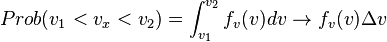 (One dimension)
The 'rightarrow' ( ) holds when the range of velocity is so small that
  is nearly uniform. The subscript on the probability distribution function,
  , will permit us to simultaneously talk about probability distributions for different variables.
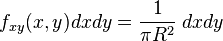
Two dimensional gas confined to within a circle
The probability density for one particle confined to a circle of radius R can be found by satisfying two criteria:
- The integral over all accessible regions of xy space is one.
- The system is ergodic if proper variables are used; we take x and y to be proper variables without proof.
Hence,
It is useful to change variables using  and
and  :
:
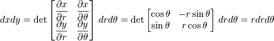
Hence,
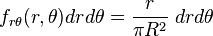
Note that rθ space is not uniformly occupied.
Kinetic energy probability distribution
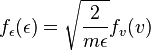
Letting E = ½mv2 equal kinetic energy, we solve for v = (2E/m)1/2the probability distribution in energy can be calculated as follows:
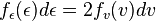
The peculiar factor of 2 occurs because two values of v contribute to the same kinetic energy. Since this is a one dimensional calculation, it is proper refer to  as kinetic energy for one degree of freedom. (In this way, a free particle in three dimensions has three degrees of freedom.) Using,
  , and a bit of algebra, it can be shown that[12]:
Maxwell's symmetry argument for velocity space
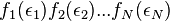
Maxwell's original derivation of the Maxwell-Boltzmann equation relied on the concept that the product of two or more independent events occurring equals the product of the probability of each event[13]. For example the probability of flipping a fair coin twice and obtaining two heads (H-H) is the product of obtain a heads one coin squared: P(H-H)=P(H)P(H) = ½·½=¼. He reasoned that for N particles, the probabilities distributions for all the particles were independent, and therefore obeyed a similar product rule:
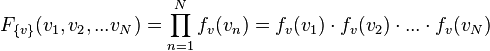
where,
![\{ v\} = [v_1, v_2, ... v_N]](../I/m/f8316d8aa71575018490fc09238f6927.png)
represents one point in a very large number of dimensions. The use of a capital letter for this 'grand' distribution function reflects the relative complexity of this space. Boltzmann also argued that the 'grand' distribution function depended only on the total energy of the gas:
 ,
,
where 
is the total energy. Ordinarily the probability distribution would also depend on density, but an ideal gas is assumed to be sufficiently tenuous that collisions have no impact except that they eventually establish thermal equilibrium. It is the total energy of an ideal gas of N particles that uniquely determines how hot it is.
Carefully redefining functions
The micro distribution functions,  , also depend only on speed, and hence only on the energy of each atom,
 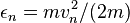 . But extreme care must be used in expressing this fact. It is safest to define a new function, g, as follows:
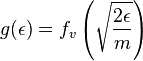 .
.
This function, g, is numerically equal to the micro distribution for a single particle, but as we shall see, is not the distribution function for the kinetic energy of an atom. Also, to be precise, it is necessary to think of  as one of two functions:
 .
.
 .
.
Velocity distribution function for a 1-D ideal gas
Using the first form, we evaluate the variation of F with  as:
as:
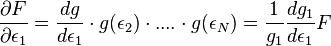 .
.
Using the second form,
 .
.
Similarly we can prove that  , which means that two expressions, each (exclusively) involving different variables are equal:
Where  is evaluated at
 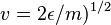 .
.
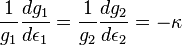
where we have yet to establish that the constant,  is a positive number. But solving this differential equation, we have:
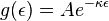
Using the ideal gas law to find kappa
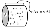
The ideal gas law is an observable fact about actual gasses. To establish that 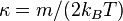 we must perform a theoretical calculation of the pressure using this distribution function. We use the fact that the distribution functions are now known (with as a parameter) and calculate the pressure exerted by this gas by employing the momentum transfer associated with elastic collisions of particles of a known density and velocity distribution off a wall, as shown in the figure. A good proof can be found in the wikibook General Chemistry[14]
Hence we have the probability distribution function for the velocity of a one-dimensional ideal gas expressed in terms of temperature:
 ,
,
where, 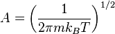 , is a normalization constant that can be found by setting
 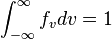 .
.
The importance of using proper phase space variables
If we change variables using the methods described above, we establish that
In other words, the wrong answer would have resulted if we assumed if this calculation had begun with slightly different (but incorrect) premise:
 . This premise is false because the transformation from the permissible phase space variables
  to energy variables introduces the factor
  .
.
The velocity distribution if the gas is confined by a potential


If this calculation is repeated for a one dimensional gas confined by a potential well,  , one obtains the following distribution function:
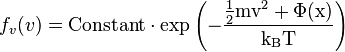 .
.
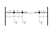
We leave it to the reader to show that a derivation of this formula follows the methods already introduced for the ideal gas. This is a significant result because the potential can be that of a harmonic oscillator  , where
  is the spring constant. Moreover, a Hamiltonian exists that describes two coupled oscillators as two uncoupled oscillators. And, this method can be extended to include a very large number of coupled oscillators[15]. In other words, a linear wave can be viewed as a classical gas of uncoupled harmonic oscillators. It was Plank's attempt to perform an thermodynamic analysis of light waves in thermal equilibrium with a closed box that lead to the breakdown of classical physics.
To be continued
The rest of this essay is presented in outline form only.
Entropy of an ideal gas
Having shown that entropy is a state variable for a monatomic ideal gas, we may use Carnot's theorem to prove that entropy is an ideal gas for all systems (otherwise the difference between Carnot cycles could violate the second law).
Carnot's theorem and the existence of entropy
Carnot's theorm ensures that the integral of dQ/T (for a reversible process) is the same regardless of what substance is inside the piston. This establishes:
- The Clausius definition of entropy, S=kʃdQ/T, does define entropy as a state variable.
- The reversible Carnot cycle permits a definition of temperature that is consistent with the definition of temperature introduced with Maxwell-Boltzmann kinetic theory of the ideal gas.
First law of thermodynamics with entropy
Now that the existence of entropy is established we may express the first law of thermodynamics in the following form:

Calculating the statistical entropy for a classical ideal gas
This section is the "punch line" to this essay.
- See the Wikipedia article on Gibbs Paradox.
The aforementioned Wikipedia link states and resolves the paradox. Following comment was made by a Wikipedia editor on the talk page to that article:
- for what it's worth, a summary of what Gibbs said:
In two different works, published thirty years apart, Gibbs remarked two different ways on how the notion of distinguishability affects entropy. I have been reading Gibbs lately and studying how he saw the issue. For the benefit of future edits on this article, I've included below direct links to Gibbs' remarks, and some interpretation of mine since Gibbs' prose can be painful to read at times.
In neither case did he find there to be an actual problem, since the correct answer fell naturally out of his mathematical formalisms. However it's evident that he saw these things as possibly tricky points for the reader, because in each case he did devote time to carefully talking about the issues.
-
On the Equilibrium of Heterogeneous Substances (1876): Internet archive copy of Part I, see section "Considerations relating to the Increase Entropy due to the Mixture of Gases by Diffusion." (starting at page 125 of the scanned file, which is page 227 of the manuscript). The key points:
- Gibbs begins by deriving (from thermodynamics) that the entropy increase by mixing two gaseous masses of different kinds, of equal volume and at constant temperature and pressure will be
 , where V is the final volume. When mixing two masses of the same kind, there is no entropy increase.
 - He emphasizes the striking property that the mixing entropy does not depend on which kinds gases are involved, whether they are very different or very similar. They only need to be of distinguishable types.
- Why entropy should increase in one case and not the other:
- "When we say that when two different gases mix by diffusion, as we have supposed, the energy of the whole remains constant, and the entropy receives a certain increase, we mean that the gases could be separated and brought to the same volume and temperature which they had at first by means of certain changes in external bodies, for example, by the passage of a certain amount of heat from a warmer to a colder body. But when we say that when two gas-masses of the same kind are mixed under similar circumstances there is no change of energy or entropy, we do not mean that the gases which have been mixed can be separated without change to external bodies. On the contrary, the separation of the gases is entirely impossible. We call the energy and entropy of the gas-masses when mixed the same as when they were unmixed, because we do not recognize any difference in the substance of the two masses. So when gases of different kinds are mixed, if we ask what changes in external bodies are necessary to bring the system to its original state, we do not mean a state in which each particle shall occupy more or less exactly the same position as at some previous epoch, but only a state which shall be undistinguishable from the previous one in its sensible properties. It is to states of systems thus incompletely defined that the problems of thermodynamics relate."
- Gibbs then goes on to consider the hypothetical situation of having two gases that are distinct (i.e. that can be later separated) but are so similar that for the dynamics of the mixing are exactly the same as the dynamics of mixing two same gases. On the atomic scale these processes would appear identical and yet the entropy would increase in one case and not the other. Gibbs says "In such respects, entropy stands strongly contrasted with energy", meaning that we cannot identify entropy with any kind of microscopic dynamics. Gibbs notes that the apparently irreversible dynamics of diffusion are not special to the distinct gas case; they are also just as well taking place in the mixing of same gases, however there is no entropy increase. To Gibbs, entropy has nothing to do with the motions of atoms but rather has to do with what we (as human observers) are able to distinguish in thermodynamic states.
- Gibbs begins by deriving (from thermodynamics) that the entropy increase by mixing two gaseous masses of different kinds, of equal volume and at constant temperature and pressure will be
-
Elementary Principles in Statistical Mechanics (1902): Gibbs' 1902 book addresses what is often called "correct Boltzmann counting". This counting is often explained as necessary to obtain extensive thermodynamics, however Gibbs introduces it in a different way (as a tool to avoid overcounting in phase space). The discussion takes place at the beginning and end of Chapter XV (transcription on Wikisource).
- Gibbs says, if an ensemble is meant to represent an actual collection of systems, then the particles in some sense must be indistinguishable because each particle needs to be copied many times. On the other hand, when the ensemble is a probability distribution used to represent the possible states of one system, we might truly speak about unique particles. At this point Gibbs notes there is nothing formally wrong with having distinguishable particles or indistinguishable particles: "The question [whether particles are indistinguishable] is one to be decided in accordance with the requirements of practical convenience in the discussion of the problems with which we are engaged."
- Classical mechanics can be done equally well with distinguishable or indistinguishable particles. When considering indistinguishable particles, Gibbs notes that for integrating over the state space, the easiest way to do it is to pretend the particles are distinguishable, then divide the phase space integral by the appropriate overcounting factor. Gibbs is not mystified by why he should divide by N!, it is simply a mathematical convenience in order to perform calculations with indistinguishable particles. If one wanted to do it the hard way, the same results could be had by integrating over phase space including each distinguishable state once and only once. "For the analytical description of a specific phase is more simple than that of a generic phase. And it is a more simple matter to make a multiple integral extend over all possible specific phases than to make one extend without repetition over all possible generic phases."
- Gibbs then goes on to make tons of calculations for the grand canonical ensemble, using the framework of indistinguishable particles. Along the line he mentions why he is focussing on indistinguishable particles: "The interest of the ensemble which has been described lies in the fact that it may be in statistical equilibrium, both in respect to exchange of energy and exchange of particles, with other grand ensembles canonically distributed and having the same values of Θ and of the coefficients μ1, μ2, etc., when the circumstances are such that exchange of energy and of particles are possible, and when equilibrium would not subsist, were it not for equal values of these constants in the two ensembles." It's worth noting that his demonstration of equilibrium would not work out using the framework of distinguishable particles: he demonstrates this in equations (514) and (515).
- At the end of the chapter he works his way towards the measure of entropy, and finally remarks on the entropy difference (in the canonical ensemble) between considering particles distinguishable or indistinguishable. At the very end of this work (and apparently the very last paragraph he published before death), Gibbs mentions a sort of mixing paradox again, but this time it is regarding extensivity:
- "For the principle that the entropy of any body has an arbitrary additive constant is subject to limitation, when different quantities of the same substance are concerned. In this case, the constant being determined for one quantity of a substance, is thereby determined for all quantities of the same substance.
To fix our ideas, let us suppose that we have two identical fluid masses in contiguous chambers. The entropy of the whole is equal to the sum of the entropies of the parts, and double that of one part. Suppose a valve is now opened, making a communication between the chambers. We do not regard this as making any change in the entropy, although the masses of gas or liquid diffuse into one another, and although the same process of diffusion would increase the entropy, if the masses of fluid were different. It is evident, therefore, that it is equilibrium with respect to generic phases, and not with respect to specific, with which we have to do in the evaluation of entropy, and therefore, that we must use the average of H or of ηgen, and not that of η, as the equivalent of entropy, except in the thermodynamics of bodies in which the number of molecules of the various kinds is constant."
- "For the principle that the entropy of any body has an arbitrary additive constant is subject to limitation, when different quantities of the same substance are concerned. In this case, the constant being determined for one quantity of a substance, is thereby determined for all quantities of the same substance.
The 1876 work was entirely concerned with thermodynamics. The Gibbs' paradox of 1876 is therefore a pure thermodynamic thing. He does allude to molecular dynamics and probabilities but that is not essential to the argument. Whether entropy increases or not is, in the end, pragmatically determined by whether we need to perform work to return the systems back to their initial thermodynamic states. As to whether the individual particles themselves are distinguishable is not relevant to his argument here: there is anyway no thought to returning each particle back to its original position (returning the systems back to their initial microscopic state) as this would anyway be impossible. Rather it is only required in thermodynamics to return the systems back to their initial thermodynamic state. For what it's worth I think the Jaynes paper does an okay job explaining and extending Gibbs' arguments here.
To sum up Gibbs' remarks in his 1902 work, Gibbs starts out by noting that classical mechanics can be done equally well with distinguishable or indistinguishable particles. Both options can be considered in classical statistical mechanics, and it is really down to the details of the system we are studying, which one we choose. Gibbs then motivates why we must use indistinguishable particles, for the study of statistical thermodynamics, as so: First of all, if they were distinguishable we could not have such an easily defined grand canonical ensemble that is in equilibrium with respect to particle exchange. Secondly, if they were distinguishable then in the canonical ensemble the average logarithm of probability would not give us a quantity behaving like entropy, when the number of particles varies. The Jaynes paper says that Gibbs' 1902 book was "the work of an old man in rapidly failing health" and that Gibbs would have written more on this paradox if he had been in better health. Perhaps true, but I suspect Gibbs didn't want to distract from the rest of the discussion in the chapter.
Are there actually two Gibbs paradoxes? Should they be called "paradoxes"? I would say yes and yes. Gibbs addressed both the mixing-of-very-similar-gasses paradox in thermodynamics, and the mixing-of-identical-gases extensivity paradox in statistical mechanics. These are two different but closely related things, and there very well may be two Gibbs paradoxes, as discussed in the article. Gibbs did not see either as an actual problem, and he never called them paradoxes, yet he did remark on them as possible places where one could make a logical error. In some sense then they really are paradoxes, along the lines of the two-envelope paradox and the Monty Hall paradox: things that can seem on the surface mysterious or counterintuitive yet which have deep down a well-defined, consistent answer.
References and such
Wikipedia...
- -defines a heat engine here.
- -describes the Stirling heat engine here.
- ↑ https://en.wikiquote.org/w/index.php?title=Thermodynamics&oldid=1642813
- ↑ https://en.wikipedia.org/w/index.php?title=History_of_entropy&oldid=577104922
- ↑ https://en.wikipedia.org/w/index.php?title=Clausius_theorem&oldid=560729049
- ↑ https://en.wikipedia.org/w/index.php?title=Entropy&oldid=584258991
- ↑ http://galileo.phys.virginia.edu/classes/252/kinetic_theory.html
- ↑ https://en.wikipedia.org/w/index.php?title=Boltzmann%27s_entropy_formula&oldid=586101028
- ↑ Robert H. Swendsen, 'Statistical mechanics of colloids and Boltzmann’s definition of the entropy' Am. J. Phys. 74 (3), March 2006
- ↑ https://en.wikipedia.org/w/index.php?title=Ergodic_hypothesis&oldid=572054479
- ↑ https://en.wikipedia.org/w/index.php?title=Perpetual_motion&oldid=584397707
- ↑ https://en.wikipedia.org/w/index.php?title=Second_law_of_thermodynamics&oldid=584405568
- ↑ "Liouville's theorem ensures that the notion of time average makes sense, but ergodicity does not follow from Liouville's theorem." https://en.wikipedia.org/w/index.php?title=Ergodic_hypothesis&oldid=572054479
- ↑ https://en.wikipedia.org/w/index.php?title=Maxwell%E2%80%93Boltzmann_distribution&oldid=581947663
- ↑ http://galileo.phys.virginia.edu/classes/252/kinetic_theory.html
- ↑ https://en.wikibooks.org/w/index.php?title=General_Chemistry/Gas_Laws&oldid=2566774.
- ↑ https://en.wikipedia.org/w/index.php?title=Normal_mode&oldid=582552032
Topic page
This topic page is for organizing the development of Statistical thermodynamics content on Wikiversity. Please, feel free to improve upon what you see; your contributions will be greatly appreciated.
Wikiversity Resources
- Topic:Statistical mechanics
- Statistical mechanics and thermodynamics (Based on probability and the counting of microstates)
- Statistical thermodynamics (Based on the Clausius definition of entropy)
- Topic:Advanced_Classical_Mechanics/Phase_Space (a work in progress that is relevant to statistical physics)
- Basic thermodynamics
- Thermodynamics and Thermodynamics_and_Equilibrium will soon be merged.
- Search for Statistical thermodynamics at Wikiversity
Wikipedia/Wikibook Resources
- Thermodynamics (Wikipedia article)
- Statistical thermodynamics (Wikipedia article)
- Category:Thermodynamics (HUGE Category of Wikipedia articles)
- StatisticalMechanics (wiki-book)
- Engineering Thermodynamics(wiki-book)
Advanced Resources
- Thermodynamics OpenCourseWare from the University of Notre Dame. A rigorous and complete upper division course. License is CC BY-NC-SA 3.0. All lectures are PDF files.
- Kittel and Kroemer's Thermal Physics. A very gentle introduction to an approach to thermodynamics which starts with statistical mechanics and then builds on those rules to derive the thermodynamical equations. This method is often much easier for physics students to understand, because you see a lot of the physical principles involved rather than just memorizing equations.
Miscellaneous
| |
Subject classification: this is a physics resource . |
| |
Resource type: this resource is a course. |
School of Physics Thermodynamics
- Classical thermodynamics
- Statistical thermodynamics
- Heat transfer
About learning projects and resources
Learning materials and learning projects can be used by multiple departments. Please cooperate with other departments that use the same learning resource. Remember, Wikiversity has adopted the "learning by doing" model for education. Lessons should center on learning activities for Wikiversity participants. Also, select a descriptive name for each learning project. Learning projects can be listed in order by Wikiversity:Naming conventions.
- See: Wikiversity learning model.
- See: Learning projects
- See: Hunter-gatherers project
- See: Learning to learn a wiki way
- See: Wikiversity:Naming conventions