Numerical Analysis/Vandermonde example

< Numerical Analysis

We'll find the interpolating polynomial passing through the three points $(1,-6)$ , $(2,2)$ , $(4,12)$ , using the Vandermonde matrix.

For our polynomial, we'll take 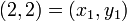$(1,-6) = (x_{0},y_{0})$ , $(2,2) = (x_{1},y_{1})$ , and $(4,12) = (x_{2},y_{2})$ .

Since we have 3 points, we can expect degree 2 polynomial.

So define our interpolating polynomial as:

$p(x) = a_{2}x^{2} + a_{1}x + a_{0}$ .

So, to find the coefficients of our polynomial, we solve the system $p(x_{i}) = y_{i}$ , $i\in \{0,1,2\}$ .

\left( \begin{array}{ccc} x_{0}^{2} & x_{0} & 1 \\ x_{1}^{2} & x_{1}& 1 \\ x_{2}^{2} & x_{2} & 1 \\ \end{array} \right) *\left( \begin{array}{c} a_{2} \\ a_{1} \\ a_{0} \end{array} \right)=\left( \begin{array}{c} y_{0} \\ y_{1} \\ y_{2} \end{array} \right)

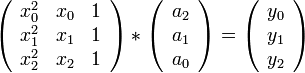
In order to solve the system, we will use an augmented matrix based on the Vandermonde matrix, and solve for the coefficients using Gaussian elimination. Substituting in our $x$ and $y$ values, our augmented matrix is:

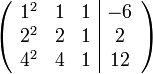
$\left( \begin{array}{ccc|c} 1^{2} & 1 & 1 & -6 \\ 2^{2} & 2 & 1 & 2 \\ 4^{2} & 4 & 1 & 12 \end{array} \right)$

Then, using Gaussian elimination,

$\left( \begin{array}{ccc|c} 1 & 1 & 1 & -6 \\ 4 & 2 & 1 & 2 \\ 16 & 4 & 1 & 12 \end{array} \right) \Rightarrow \left( \begin{array}{ccc|c} 1 & 1 & 1 & -6 \\ 0 & -2 & -3 & 26 \\ 0 & -12 & -15 & 108 \end{array} \right) \Rightarrow \left( \begin{array}{ccc|c} 1 & 1 & 1 & -6 \\ 0 & -2 & -3 & 26 \\ 0 & 0 & 3 & -48 \end{array} \right) \Rightarrow \left( \begin{array}{ccc|c} 1 & 1 & 0 & 10 \\ 0 & 2 & 0 & -22 \\ 0 & 0 & 1 & -16 \end{array} \right) \Rightarrow \left( \begin{array}{ccc|c} 1 & 0 & 0 & -1 \\ 0 & 1 & 0 & 11 \\ 0 & 0 & 1 & -16 \end{array} \right)$

Our coefficients are $a_{2} = -1$ , $a_{1} = 11$ , and $a_{0} = -16$ . So, the interpolating polynomial is

$p(x) = -x^{2} +11x -16$ .

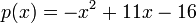Adding a point

Now we add a point, 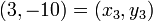$(3,-10) = (x_{3},y_{3})$ , to our data set and find a new interpolation polynomial with this method.

Since we have 4 points, we will have degree 3 polynomial.

Thus Our polynomial is $p(x) = a_{3}x^{3} + a_{2}x^{2} + a_{1}x + a_{0}$ ,

and we get the coefficients by solving the system $p(x_{i}) = y_{i}$ .

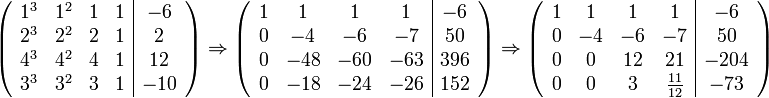
Constructing our augmented matrix as before and using Gaussian elimination, we get:

$\left( \begin{array}{cccc|c} 1^{3} & 1^{2} & 1 & 1 & -6 \\ 2^{3} & 2^{2} & 2 & 1 & 2 \\ 4^{3} & 4^{2} & 4 & 1 & 12 \\ 3^{3} & 3^{2} & 3 & 1 & -10 \end{array} \right) \Rightarrow \left( \begin{array}{cccc|c} 1 & 1 & 1 & 1 & -6 \\ 0 & -4 & -6 & -7 & 50 \\ 0 & -48 & -60 & -63 & 396 \\ 0 & -18 & -24 & -26 & 152 \end{array} \right) \Rightarrow \left( \begin{array}{cccc|c} 1 & 1 & 1 & 1 & -6 \\ 0 & -4 & -6 & -7 & 50 \\ 0 & 0 & 12 & 21 & -204 \\ 0 & 0 & 3 & \frac{11}{12} & -73 \end{array} \right)$

$\Rightarrow \left( \begin{array}{cccc|c} 1 & 1 & 1 & 1 & -6 \\ 0 & -4 & -6 & -7 & 50 \\ 0 & 0 & 12 & 21 & -204 \\ 0 & 0 & 0 & \frac{1}{4} & -22 \end{array} \right) \Rightarrow \left( \begin{array}{cccc|c} 1 & 1 & 1 & 0 & 82 \\ 0 & -4 & -6 & 0 & -566 \\ 0 & 0 & 12 & 0 & 1644 \\ 0 & 0 & 0 & 1 & -88 \end{array} \right) \Rightarrow \left( \begin{array}{cccc|c} 1 & 1 & 0 & 0 & -55 \\ 0 & -4 & 0 & 0 & 256 \\ 0 & 0 & 1 & 0 & 137 \\ 0 & 0 & 0 & 1 & -88 \end{array} \right)$

$\Rightarrow \left( \begin{array}{cccc|c} 1 & 0 & 0 & 0 & 9 \\ 0 & 1 & 0 & 0 & -64 \\ 0 & 0 & 1 & 0 & 137 \\ 0 & 0 & 0 & 1 & -88 \end{array} \right)$

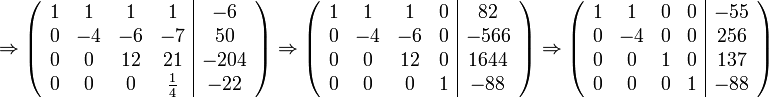
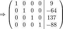
Therefore, our polynomial is:

$p(x) = 9x^{3} -64x^{2} + 137x -88$ .

This article is issued from Wikiversity - version of the Saturday, April 02, 2016. The text is available under the Creative Commons Attribution/Share Alike but additional terms may apply for the media files.