Numerical Analysis/Newton form example
< Numerical AnalysisWe'll find the interpolating polynomial passing through the points  ,
,  ,
,  , using the Newton form of the interpolation polynomial.
The Newton form is given by the formula 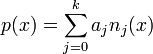 , where
 ![a_{j} = [y_{0},\ldots,y_{j}]](../I/m/02851bbd99428eedd1e38ae8c9d8484d.png) and
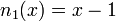
and 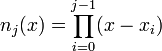 , with
  . We start by finding each
  .
.

Next, we find the necessary divided differences. First, ![[y_{0}] = -6](../I/m/119345f372da6a8eab48f9aaf6075f2e.png) ,
, ![[y_{1}] = 2](../I/m/5d397d75c94772f0f6dac98f4eba7f80.png) , and
, and ![[y_{2}] = 12](../I/m/29bb7074521956f6ba31bb24dc44f121.png) . For the next level, we have:
. For the next level, we have:
![[y_{0},y_{1}] = \frac{2+6}{2-1} = 8](../I/m/4b8b3cd02cff9f469800e5889283ece6.png)
![[y_{1},y_{2}] = \frac{12-2}{4-2} = 5](../I/m/a5ee1772350a6d3d17325c602e4bc599.png)
Finally, we can find:
![[y_{0},y_{1},y_{2}] = \frac{5-8}{4-1} = -1](../I/m/a7907e5ca6dfc3d443a13fefc651fb20.png) .
.
Now, we can find the coefficients  .
.
![a_{0} = [y_{0}] = -6](../I/m/4ec07dd5f77061743e7133896176b08c.png)
![a_{1} = [y_{0},y_{1}] = 8](../I/m/556b78da78a8c6f6acea8f66e7dbcff0.png)
![a_{2} = [y_{0},y_{1},y_{2}] = -1](../I/m/5fd6f6ef6fa58d27fc3b6e30f43d44d4.png)
Substituting and simplifying, we get our interpolating polynomial:
 .
.
Adding a point
Now let's add the point  to our data set and find the new polynomial using the same method. Due to the formula for the Newton form, we only have to add the term
  to our previous interpolating polynomial.
First, we have
 .
.
Now to find  we calculate some more divided differences.
![[y_{3}] = -10](../I/m/a5cb07608bf774e510fe98b8a2843bba.png)
![[y_{2},y_{3}] = \frac{-10-12}{3-4} = 22](../I/m/3f92fd9f08b0dc02ee811c5960e73987.png)
![[y_{1},y_{2},y_{3}] = \frac{22-5}{3-2} = 17](../I/m/748040eca2fbe6f1d4f0033af25e07eb.png)
![a_{3} = [y_{0},\ldots,y_{3}] = \frac{17+1}{3-1} = 9](../I/m/437872d00068939725f0a384853ac058.png)
So, our new interpolating polynomial is:
 .
.