Numerical Analysis/stability of RK methods
< Numerical AnalysisDefinitions
let  is the local truncation error, and k is the number of time steps, then:
- The numerical method is consistent with a differential equation if
-
 over
over  .
.
according to this definition w:Euler's method is consistent.
-
- A numerical method is said be convergent with respect to differential equation if
 over ;
where
 is the approximation for
  .
. - A numerical method is stable if small change in the initial conditions or data, produce a correspondingly small change in the subsequent approximations.
Theorem: For an initial value problem
-
 with
with ![t\in[t_0,t_0+\alpha]](../I/m/63c60ccd0927bfd8de2aa6833425c8e2.png)
and certain initial conditions,  , let us consider a numerical method of the form
 and
and  .
.
If there exists a value  such that it is continuous on the iterative domain,
  and if there exists an
  such that
 for all
  ,
,
the method fulfills the w:Lipschitz condition, and it is stable and convergent if and only if it is consistent. That is,
-
 for all
  .
.
For a similar argument, one can deduce the following for multi- step methods:
- The method is stable if and only if all roots,
 , of the characteristic polynomial satisfy
-
 ,
,
and any root of
is simple root.
-
- one more result is that if the method is consistent with the differential equation, the method is stable if and only if it it is convergent.

stability polynomials of Runge-Kutta methods
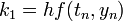
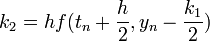
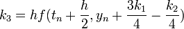
The w:Runge–Kutta methods are very useful in solving systems of differential equations, it has wide applications for the scientists and the engineers, as well as for the economical models, the recognized with their practical accuracy where we can use and get very good results and approximations when solving an ODE problem, RK has the general form :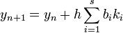 , where
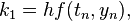


such that
- s is the number of stages,
- aij (for 1 ≤ j < i ≤ s),
- bi (for i = 1, 2, ..., s)
- and ci (for i = 2, 3, ..., s).
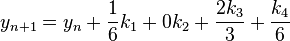
Example:finding the stability polynomial for RK4's methods
for RK4" case ", which characterizes by
  which has the form: the stability region is found by applying the method to the linear test equation
- the stability region is found by applying the method to the linear test equation

using the linearized equation  , we get

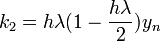

substitue these back in  , yields
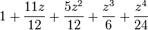
![y_{n+1} = [1+(h\lambda)+\frac{(h\lambda)^2}{2}+\frac{(h\lambda)^3}{6}+\frac{(h\lambda)^4}{24}]y_n=R(h\lambda)y_n](../I/m/023b1a1f3fb7b48ba026ab524f5bda23.png)
- and so the characteristic polynomial
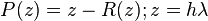 for the absolute stability region for this method, set |R(z)|<1,
and so we get the region in figue1. case
for the absolute stability region for this method, set |R(z)|<1,
and so we get the region in figue1. case
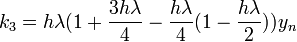
the table below shows the final forms for the stability function for different forms of RK4, these RK4's are different in the values of  , and they are fullfilling the consistencty requirement for the method i.e :
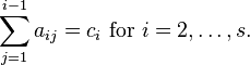
case#  |
stability function |
caseI  |
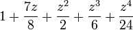 |
caseII_a  |
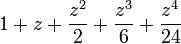 |
| caseII_b |
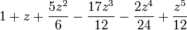 |
caseIII 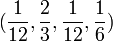 |
 |
| caseIV |
|
classical Rk  |
|
Plotting the stability region
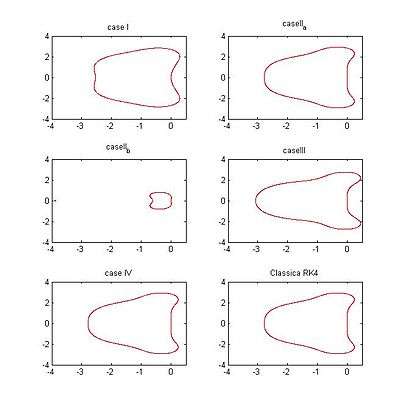
In order to plot the stability region, we can set the stability function to be bounded by 1 and solve for the values of z, then draw z in the complex plane. Since R(z) is the unit circle in the complex plane, each point on the boundary can be represented as  and so by changing
  over the interval
![[0,2\pi]](../I/m/58c9a5de0cb1a343ae0acd1fb191eea1.png) , we can draw the boundaries of that region. The following w:OCTAVE/Matlab code does this by plotting contour curves until reaching the boudaries:
, we can draw the boundaries of that region. The following w:OCTAVE/Matlab code does this by plotting contour curves until reaching the boudaries:
[x,y] = meshgrid(-6:0.01:6,-6:0.01:6);
z = x+i*y;
R = 1+z+0.5*z^2+(1/6)*z^3+(1/24)*z^4;
zlevel = abs(R);
contour(x,y,zlevel,[1 1]);
The figure at right shows the absolute stability regions for RK4 cases which is tabulated above
References
- Eberly, David (2008), stability analysis for systems of defferential equation.
- Ababneh, Osama; Ahmad, Rokiah; Ismail, Eddie (2009), "on cases of fourth-order Runge-Kutta methods", European journal of scientific Research.
- Mathews, John; Fink, Kurtis (1992), numerical methods using matlab.
- Stability of Runge-Kutta Methods