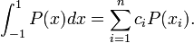
Numerical Analysis/Gaussian Quadrature

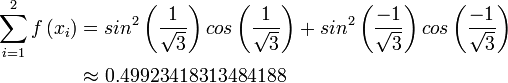
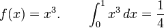
< Numerical Analysis

For the first example, I just want an example to show that the solution is exact for polynomials of degree $2n-1$ , using the $n$ th degree Legendre polynomial. I'm going to approximate $\int_{-1}^1 x^3 dx$ .

$\begin{align} \int_{-1}^1 x^3 dx & = \left(\frac{1}{\sqrt{3}}\right)^3 + \left(\frac{-1}{\sqrt{3}}\right)^3 \\ \frac{1}{4} 1^4 - \frac{1}{4} (-1)^4 & = \left(\frac{1}{3\sqrt{3}}\right) - \left(\frac{1}{3\sqrt{3}}\right) \\ \frac{1}{4} - \frac{1}{4} &= 0 \end{align}$

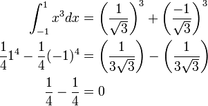
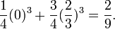
This problem accurately illustrates the method for solving problems using the Gaussian Quadrature algorithm. Note that the zeros of the Legendre polynomials of degree $n$ are $\frac{1}{\sqrt{3}}$ and $-\frac{1}{\sqrt{3}}$ .

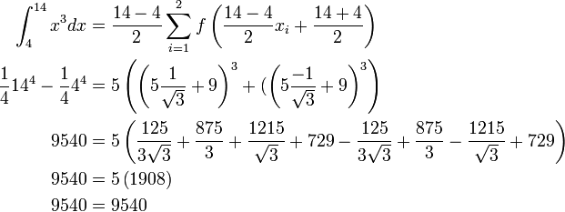
We can see from the previous example that this method works quite well if we are integrating from $-1$ to $1$ , but in application, we rarely want to integrate over such a simple region. So in our next example, we will show that this technique is also effective if we change the limits of integration, as seen on the Wikipedia page, then we will solve the example $\int_4^{14} x^3 dx$

$\begin{align} \int_4^{14} x^3 dx &= \frac{14-4}{2} \sum_{i=1}^2 f\left(\frac{14-4}{2} x_i + \frac{14+4}{2}\right) \\ \frac{1}{4} 14^4 - \frac{1}{4} 4^4 &= 5 \left(\left(5\frac{1}{\sqrt{3}} + 9\right)^3 +(\left(5\frac{-1}{\sqrt{3}} + 9\right)^3\right) \\ 9540 &= 5 \left(\frac{125}{3\sqrt{3}} + \frac{875}{3} + \frac{1215}{\sqrt{3}} + 729 - \frac{125}{3\sqrt{3}} + \frac{875}{3} - \frac{1215}{\sqrt{3}} + 729\right) \\ 9540 &= 5\left(1908\right)\\ 9540 &= 9540 \end{align}$

We will next show how to solve a problem that isn't a simple polynomial. We will approximate $\int_{-1}^1 e^x dx$ using a two point Gaussian approximation, and discuss the error analysis.

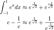
$\begin{align} \int_{-1}^1 e^x dx &\approx e^{\frac{1}{\sqrt{3}}} + e^{\frac{-1}{\sqrt{3}}} \\ e - \frac{1}{e} &\approx e^{\frac{1}{\sqrt{3}}} + \frac{1}{e^{\frac{1}{\sqrt{3}}}} \end{align}$

We will next analyze this error, looking at the actual error followed by finding the error bound. We denote the approximation by $f_{approx}$ and the exact solution by $f_{exact}$ .

$\begin{align} \left|f_{exact} - f_{approx}\right| &= \left|e - \frac{1}{e} - e^{\frac{1}{\sqrt{3}}} - \frac{1}{e^{\frac{1}{\sqrt{3}}}}\right| \\ &= 0.00770629937787233598077 \end{align}$

The theoretical error bound when using the Legendre polynomial method is

$\begin{align} \left|f_{exact}-f_{approx}\right| &\le \frac{(b-a)^{2n+1}(n!)^4}{(2n+1)\left[(2n)!\right]^3} f^{(2n)}\left(\xi\right), a<\xi<b \\ &\le \frac{2^5 2^4}{5*4!^3} e \\ &= \frac{2^9}{5*24^3} e \\ &= 0.02013542095154848322489 \end{align}$

In our example, the actual error was well within the error bound. We also see that with only two calculations, this is a very good algorithm for approximating integrals quickly with relatively good accuracy.

Exercises

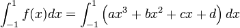
1. Show that Gaussian Quadrature can solve exactly general cubic polynomials.

a) Set up the integral:

Solution:

$\int_{-1}^1 f(x) dx = \int_{-1}^1 \left(ax^3 +bx^2 + cx + d\right) dx$

b) Evaluate the integral:

Solution:

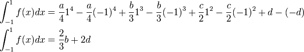
$\begin{align} \int_{-1}^1 f(x) dx &= \frac{a}{4} 1^4 - \frac{a}{4} (-1)^4 + \frac{b}{3} 1^3 - \frac{b}{3} (-1)^3 + \frac{c}{2} 1^2 - \frac{c}{2} (-1)^2 + d - (-d)\\ \int_{-1}^1 f(x) dx &= \frac{2}{3} b + 2d \end{align}$

c) Evaluate the approximation:

Solution:

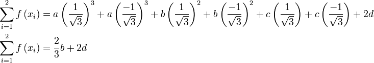
$\begin{align} \sum_{i=1}^2 f\left(x_i\right) &= a\left(\frac{1}{\sqrt{3}}\right)^3 + a\left(\frac{-1}{\sqrt{3}}\right)^3 + b\left(\frac{1}{\sqrt{3}}\right)^2 + b\left(\frac{-1}{\sqrt{3}}\right)^2 + c \left(\frac{1}{\sqrt{3}}\right) + c\left(\frac{-1}{\sqrt{3}}\right) + 2d\\ \sum_{i=1}^2 f\left(x_i\right) &= \frac{2}{3}b + 2d \end{align}$

d) Do parts b and c correspond?

Solution:

Yes

2. Approximate 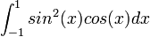$\int_{-1}^1 sin^2(x) cos(x) dx$ using Gaussian Quadrature

a) Evaluate the problem symbolically:

Solution:

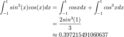
$\begin{align} \int_{-1}^1 sin^2(x)cos(x) dx &= \int_{-1}^1 cos x dx + \int_{-1}^1 cos^3 x dx \\ &= \frac{2 sin^3(1)}{3} \\ &\approx 0.397215491060637 \end{align}$

b) Evaluate the approximation:

Solution:

$\begin{align} \sum_{i=1}^2 f\left(x_i\right) &= sin^2\left(\frac{1}{\sqrt{3}}\right) cos\left(\frac{1}{\sqrt{3}}\right) + sin^2\left(\frac{-1}{\sqrt{3}}\right) cos\left(\frac{-1}{\sqrt{3}}\right) \\ &\approx 0.49923418313484188 \end{align}$

c) Find the actual error

Solution:

$\left|f_{exact} - f_{approx}\right| \approx 0.102018692074204$

d) Find the error bound

Solution:

$\begin{align} \left|f_{exact}-f_{approx}\right| &\le \frac{(b-a)^{2n+1}(n!)^4}{(2n+1)\left[(2n)!\right]^3} f^{(2n)}\left(\xi\right), a<\xi<b \\ &\le \frac{2^5 2^4}{5*4!^3} f^4(\xi) \\ &\le \frac{2^9}{5*24^3} * 20.1824 \\ &\le 0.14949925 \end{align}$

d) Is the actual error less than the error bound?

Solution:

Yes

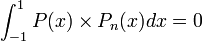
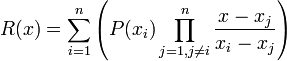
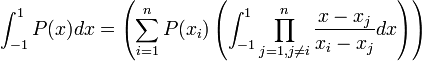
3. If $x_1, x_2,...., x_n$ are the roots of the $n$ th Legendre Polynomial $P_n(x)$ and that for each $i=1,2,....,n$ , the numbers $c_i$ are defined by

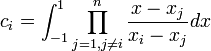
$c_i = \int_{-1}^1 \prod_{j=1,j\neq i}^n \frac{x-x_j}{x_i-x_j} dx$

Prove that if $P(x)$ is any polynomial of degree less than $2n$ , then

$\int_{-1}^1 P(x) dx = \sum_{i=1}^n c_i P(x_i).$

Proof:

The set that is relevant to this proof is the set of Legendre Polynomials, a collection orthogonal polynomials ${P_0(x), P_1(x),...,P_n(x),...,}$ with properties:

For each $n, P_n(x)$ is a monic polynomial of degree $n$ .
$\int_{-1}^1 {P(x)}\times{P_n(x)}dx = 0$ whenever $P(x)$ is a polynomial of degree less that $n$ .

First we use polynomial division, to get 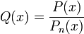$Q(x) = \frac{P(x)}{P_n(x)}$ with a remainder term $R(x)$ , so that $P(x) = Q(x)\times P_n(x) + R(x)$ and the two polynomials $Q(x)$ and $R(x)$ are of degree less than $n$ and $P_n(x)$ is of degree $n$ . Then using this fact we can rewrite the original integral into the form

\int_{-1}^1 P(x)dx = \int_{-1}^1 {P_n(x)}\times{Q(x)}dx + \int_{-1}^1 R(x)dx

Since the degree of $P(x)$ is less than twice the degree of the w: Legendre polynomial, then the degree of $Q(x)$ is less than the degree of $P_n(x)$ . So (by Legendre property 2 started above), 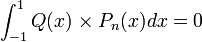$\int_{-1}^1 Q(x)\times P_n(x) dx = 0$ . Thus we see that 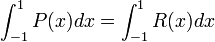$\int_{-1}^1 P(x) dx = \int_{-1}^1 R(x) dx$ . We do not know what $R(x)$ is, but we know it has degree less than $n$ so it equals the polynomial that interpolates it at the values $x_1, x_2,...., x_n$ . We will use the w: Lagrange polynomial form. Since $x_i$ is a roots of $P_n$ for each $i= 1, 2, ..., n$ , we have

P(x_i) = Q(x_i)\times P_n(x_i) + R(x_i)= Q(x_i)\times 0 + R(x_i)= R(x_i)

Since $R(x)$ is a polynomial of degree less than $n$ , then Lagrange polynomial for $R(x)$ is

R(x) = \sum_{i=1}^n \left(P(x_i) \prod_{j=1,j\neq i}^n \frac{x-x_j}{x_i-x_j}\right)

We next integrate this polynomial by

\int_{-1}^1 P(x) dx = \int_{-1}^1 R(x) dx = \int_{-1}^1 \left(\sum_{i=1}^n \left(P(x_i) \prod_{j=1,j\neq i}^n \frac{x-x_j}{x_i-x_j}\right)\right) dx

Since $P(x_i)$ is a constant, we will pull that outside the integral, giving us

\int_{-1}^1 P(x) dx = \left(\sum_{i=1}^n P(x_i)\left(\int_{-1}^1 \prod_{j=1,j\neq i}^n \frac{x-x_j}{x_i-x_j} dx\right)\right)

We then note that

c_i = \int_{-1}^1 \prod_{j=1,j\neq i}^n \frac{x-x_j}{x_i-x_j} dx

so we will substitute $c_i$ into our integration, giving us

\int_{-1}^1 P(x) dx = \sum_{i=1}^n c_i P(x_i).

This completes the proof.

Gaussian Quadrature Example

I realized that there was insufficient information after the derived and solved sample on Gaussian Quadrature thus i took the pain to edit this wikiversity page by adding a solved example to the information already on there and below is what i factored in.

Find the constants C_0, C_1, and x_1 so that the quadrature formula

\int_{0}^1 f (x)\,dx = C_0 f(0)+ C_1 f(x_1).

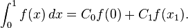
has the highest possible degree of precision.

Solution

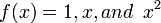
Since there are three unknowns, C_0, C_1 and x_1, we will expect the formula to be exact for

f (x) = 1, x, and \, \ x^2

Thus

f (x)= 1,\ \int_{0}^1 f (x)\,dx= 1 = C_0 + C_1\ \qquad \ Equation 1, \qquad f (x)= x,\ \int_{0}^1 f (x)\,dx= \frac{1}{2} = C_1x_1\ \qquad \ Equation 2. \qquad f (x)= x^2,\ \int_{0}^1 f (x)\,dx= \frac{1}{3} = C_1x_1^2.

Equation 2 and 3 will yield.

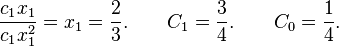
\frac{c_1x_1}{c_1x_1^2} = x_1 = \frac{2}{3}. \qquad C_1=\frac{3}{4}. \qquad C_0= \frac{1}{4}.

Hence

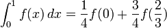
\int_{0}^1 f (x)\,dx = \frac{1}{4}f(0)+ \frac{3}{4}f(\frac{2}{3})

Now,

f(x)=x^3.\qquad \int_{0}^1 x^3\,dx = \frac{1}{4}

And

\frac{1}{4}(0)^3 + \frac{3}{4}(\frac{2}{3})^3=\frac{2}{9}.

Thus the degree of the precision is 2

Example Quiz

	By convention for consistency
	Because Legendre polynomials of degree $n$ are orthogonal to any other polynomial with degree less than $n$
	Because they make $f(x) = 0$ when approximating $f(x)$
	None of these

	True
	False

	10.56
	0
	4.13
	50.25

	5.85
	0.13
	28.83
	12.44

	The $n$ th derivative of $f(x)$ must be nonzero
	$f(x)$ is discontinuous over the range of integration
	$f(x)$ is constant over the range
	The method never fails, it just can suffer from poor accuracy

Your score is 0 / 0

This article is issued from Wikiversity - version of the Saturday, April 02, 2016. The text is available under the Creative Commons Attribution/Share Alike but additional terms may apply for the media files.