Linear algebra
Material covered in these notes are designed to span over 12-16 weeks. Each subpage will contain about 3 hours of material to read through carefully, and additional time to properly absorb the material.
Introduction - Linear Equations
In this course we will investigate solutions to linear equations, vectors and vector spaces and connections between them.
Of course you're familiar with basic linear equations from Algebra. They consist of equations such as
 .
.
and you're hopefully familiar with all the usual problems that go along with this sort of equation. Such as how to find the slope, how to place the equation in point-slope form, standard form, or slope-intercept form.
All of these ideas are useful, but we will, at first, be interested in systems of linear equations. A system of equations is some collection of equations that are all expected to hold at the same time. Let us start with an example of such a system.
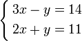 .
.
Usually the first questions to ask is are there any solutions to a system of equations. By this we mean is there a pair of numbers so that both equations hold when you plug in this pair. For example, in the above system, if you take  and
and  then you can check that both equations hold for this pair of numbers:
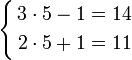 .
.
Notice that we are asking for the same pair of numbers to satisfy both equations. The first thing to realize is that just because you ask for two equations to hold at the same time doesn't mean it is always possible. Consider the system:

Clearly there is a problem. If  and
and  then you would have
 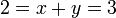 , and so
  . Which is absurd. Just because we would like there to be a pair of numbers that satisfy both equations doesn't mean that we will get what we like. One of the main goals of this course will be to understand when systems of equations have solutions, how many solutions they have, and how to find them.
In the first example above there is an easy way to find that and is the solution directly from the equations.
If you add these two equations together, you can see that the y's cancel each other out. When this happens, you will get  , or . Substituting back into the above, we find that . Note that this is the only solution to the system of equations.
Frequently one encounters systems of equations with more then just two variables. For example one may be interested in finding a solution to the system:
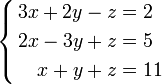 .
.
Solving Linear Systems Algebraically
One was mentioned above, but there are other ways to solve a system of linear equations without graphing.
Substitution
If you get a system of equations that looks like this:


You can switch around some terms in the first to get this:

Then you can substitute that into the bottom one so that it looks like this:


Then, you can substitute 2 into an x from either equation and solve for y. It's usually easier to substitute it in the one that had the single y. In this case, after substituting 2 for x, you would find that y = 7.
Thinking in terms of matrices
Much of finite elements revolves around forming matrices and solving systems of linear equations using matrices. This learning resource gives you a brief review of matrices.
Matrices
Suppose that you have a linear system of equations
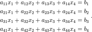
Matrices provide a simple way of expressing these equations. Thus, we can instead write
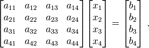
An even more compact notation is
![\left[\mathsf{A}\right] \left[\mathsf{x}\right] = \left[\mathsf{b}\right] ~~~~\text{or}~~~~ \mathbf{A} \mathbf{x} = \mathbf{b} ~.](../I/m/9ab65143e05a0e68423b953fbc300fc3.png)
Here  is a
is a  matrix while
  and
and  are
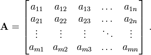
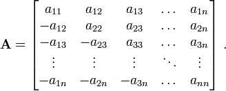
are  matrices. In general, an
  matrix is a set of numbers
arranged in
matrix is a set of numbers
arranged in  rows and
  columns.
Practice Exercises
Practice: Expressing Linear Equations As Matrices
Types of Matrices
Common types of matrices that we encounter in finite elements are:
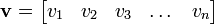
- a row vector that has one row and columns.
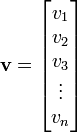
- a column vector that has rows and one column.
- a square matrix that has an equal number of rows and columns.
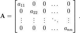
- a diagonal matrix which is a square matrix with only the
diagonal elements ( ) nonzero.
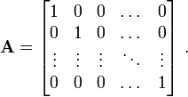
- the identity matrix (
 ) which is a diagonal matrix and
with each of its nonzero elements () equal to 1.
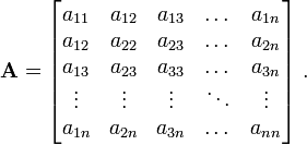
- a symmetric matrix which is a square matrix with elements
such that  .
.
- a skew-symmetric matrix which is a square matrix with elements
such that  .
.
Note that the diagonal elements of a skew-symmetric matrix have to be zero:  .
.
Matrix addition
Let and  be two matrices with components
  and
and  , respectively. Then

Multiplication by a scalar
Let be a matrix with components and let
 be a scalar quantity. Then,

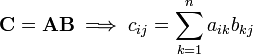
Multiplication of matrices
Let be a matrix with components . Let be a  matrix with components .
The product  is defined only if
  . The matrix
  is a
is a  matrix with components
  . Thus,
Similarly, the product  is defined only if
  . The matrix
  is a
is a  matrix with components
  . We have
Clearly,  in general, i.e., the matrix product is not
commutative.
in general, i.e., the matrix product is not
commutative.
However, matrix multiplication is distributive. That means

The product is also associative. That means

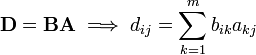
Transpose of a matrix
Let be a matrix with components . Then the transpose of the matrix is defined as the  matrix
  with components
  . That is,
An important identity involving the transpose of matrices is

Determinant of a matrix
The determinant of a matrix is defined only for square matrices.
For a  matrix , we have

For a  matrix, the determinant is calculated by expanding into
minors as
matrix, the determinant is calculated by expanding into
minors as
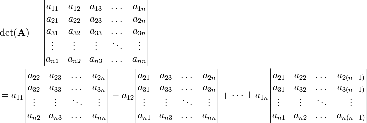
In short, the determinant of a matrix has the value
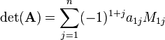
where  is the determinant of the submatrix of formed
by eliminating row
is the determinant of the submatrix of formed
by eliminating row  and column
  from .
Some useful identities involving the determinant are given below.
- If is a matrix, then

- If is a constant and is a matrix, then

- If and are two matrices, then

If you think you understand determinants, take the quiz.
Inverse of a matrix
Let be a matrix. The inverse of is denoted by  and is defined such that

where is the identity matrix.
The inverse exists only if  . A singular matrix
does not have an inverse.
. A singular matrix
does not have an inverse.
An important identity involving the inverse is

since this leads to:

Some other identities involving the inverse of a matrix are given below.
- The determinant of a matrix is equal to the multiplicative inverse of the
determinant of its inverse.

- The determinant of a similarity transformation of a matrix
is equal to the original matrix.

We usually use numerical methods such as Gaussian elimination to compute the inverse of a matrix.
Eigenvalues and eigenvectors
A thorough explanation of this material can be found at Eigenvalue, eigenvector and eigenspace. However, for further study, let us consider the following examples:
- Let :
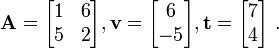
Which vector is an eigenvector for ?
We have
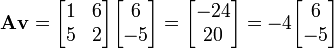 , and
, and 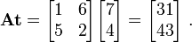
Thus,  is an eigenvector.
- Is
 an eigenvector for
 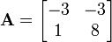 ?
?
We have that since 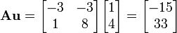 , is not an eigenvector for
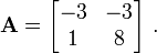
Resources
Wikipedia
Wikibooks
External links
- OER Matrices content at Wikieducator
- MIT 18.06 Linear Algebra, Spring 2005 - Video Lecture
- Khan Academy Linear Algebra videos
- Interactive online programs and Linear Algebra tutorial