Advanced Classical Mechanics/Phase Space

< Advanced Classical Mechanics

Phase space refers to the plotting of both a particle's momentum and position on a two dimensional graph. It also refers to the tracking of N particles in a 2N dimensional space. In many cases, the coordinates used are the canonical variables of Hamiltonian mechanics. If these canonical variables are used, the motion of particles in phase space exhibits properties that lead to important results in the field of thermodynamics and statistical mechanics.

How phase spaces are used

Phase space can describe the orbit of one particle, or the orbits of a large number of particles. It can even be used to describe a large number of collections of N particles, where N itself is a large number. Finally phase space can be used to describe the probability distributions of how collections of N particles behave if they are allowed to exchange particles and energy with the universe.

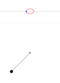
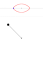
Single particle confined to one dimension creates a 2-dimensional phase space

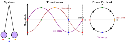
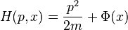
Fig. 1a. (from Wikipedia article Phase Space) A phase space of position and velocity for a simple pendulum.

The most elementary phase space consists of a single particle confined to one dimensional motion, under the influence of a conservative force field. Such a system can be modeled using Hamiltonian methods. A suitable Hamiltonian is the total energy, expressed as a function of position, x, and momentum, p:

H(p,x) = \frac{p^2}{2m}+ \Phi(x)

From w:Hamiltonian mechanics we have these equations of motion:

\frac{dx}{dt}=\frac{\partial H}{\partial p}

, and

\frac{dp}{dt}=-\frac{\partial H}{\partial x}

, and

dH/dt =\partial H/\partial t

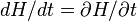
Newton's equations of motion follow immediately: 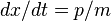$dx/dt =p/m$ , and $dp/dt = -\partial\Phi/\partial x$ , and $dE/dt =\partial H/\partial t$ .

Figure 1b. Animations showing the motion in phase space for a pendulum.

Pendulum with an initial angle of 45°
Pendulum with an initial angle of 135°
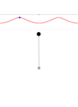
Pendulum with enough energy for a full swing

N non-interacting or weakly interacting particles

Fig. 3. Motion in phase space of for uniformly accelerated motion. Shown are a region of phase space at two different times. Initially, x and p are close to zero. Later both x and p have increased. Note how the shape changes, but the area is preserved.

Fig. 4. The area (in black) is conserved, but the motion in phase space is more chaotic.

A collection of N non-interacting particles is also a microcanonical ensemble of individual particles. Three particles constrained to one dimension can often serve as a model for a single particle in the three spatial dimensions (xyz). For this reason, these 'particles' are often referred to as w:degrees of freedom (dof).

If the potential is constant (i.e. $\Phi(x, y, z) =0$ we have a crude model of gas called an ideal gas. The model is crude because no attempt has been made to model any interaction between these particles. An important variation is an ensemble of non-interacting particles where it is assumed that some process has randomized the orbits. A collection of N non-interacting particles confined to one dimension is isomorphic to a collection of N/3 particles in xyz space (if N/3 is an integer). Figure 2 (to the left) shows a collection of non-interacting particles confined by a potential well. The initial state is not randomized, but instead have been artificially arranged to fill rectangle in phase space. The time evolution of this initial configuration is displayed as an animation.

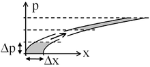
The figures to the right depict this motion by showing the region occupied in phase space at time, t=0, and at some time later. Figure 3 depicts the phase space of a particle that experiences a constant force. The initial configuration fills a region of phase space that includes a particle at rest at the origin (lower left corner of the shaded shape. This initial region includes a small initial displacement (up to approximately Δx) as well as a small initial momentum (up to approximately Δp). As time evolves, these particles, initially near the origin and nearly at rest, will accelerate. The second grey shape of Figure 3 shows these particles at a later instant in time.

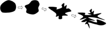
Figure 4 illustrates how weak interactions might cause the shape in phase space to randomize. The behavior shown in the figure is more a schematic that representative of typical cases. There is probably no such thing as 'typical' behavior associated with complicated systems. But if the system is described by Hamiltonian equations, then the area is conserved if the phase space has only two dimensions. In higher dimensions, the volume (more properly called hypervolume) is preserved if the system is Hamiltonian.

Friction and phase space

Fig. 5. (a) The undamped simple harmonic oscillator (Q=

\infty

) can be modeled by a Hamiltonian. (b) If friction is present, the oscillator is damped (Q=3), the area is not conserved, and the system cannot be modeled using Hamiltonian equations.

Whether or not friction exists has profound effects on how a system is modeled. Figure 5a shows the undamped simple harmonic oscillator, which is described by the Hamiltonian 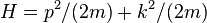$H=p^2/(2m)+ k^2/(2m)$ , where $k$ is the spring constant. Figure 5a represents the microscopic world where friction does not exist as we know it. Figure 5b reflects the macroscopic world we see and live in, where friction is everywhere and unavoidable.

It is interesting ponder the following two facts about Figures 5a and 5b:

If a macroscopic mass and spring followed the idealized, frictionless, and Hamiltonian model of Figure 5a, it would be a perpetual motion machine of the third kind.
If a collection of isolated atoms did not follow the idealized, frictionless, and Hamiltonian model of Figure 5a, the atoms would spontaneously lose energy. The corresponding reduction of temperature would permit the construction of a perpetual motion machine of the second kind, also

Both perpetual motion machines are considered impossible to achieve^[1].

Liouville's theorem

Liouville's theorem applies only to Hamiltonian systems. The Hamiltonian is allowed to vary with time, and there are no restrictions regarding how strongly the degrees of freedom are coupled^[2]^[3]. Liouville's theorem states that:

The density of states in an ensemble of many identical states with different initial conditions is constant along every trajectory in phase space.

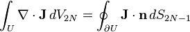
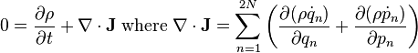
It states that if one constructs an ensemble of paths, the probability density along the trajectory remains constant. To prove this we use the generalized Stokes' Theorem to equate the n-dimensional volume integral of the divergence of a vector field J over a region U to the (n-1)-dimensional surface integral of J over the boundary of U^[4]^[5]^[6]^[7]:

\int_U \nabla \cdot \mathbf{J} \, dV_{2N} = \oint_{\partial U} \mathbf{J} \cdot \mathbf{n} \, dS_{2N-1}

Let $n=2N$ represent all the dimensions of phase space, and let the $2N$ dimensional vector field. Define $\mathbf{J}$ as the 'current' of particles in phase space, and $\rho$ is the density (number of particles per unit 2N-dimensional hypersphere. (The dots represent differentiation with respect to time.)

\mathbf{J} =[\dot q_1 , \dot p_1 , \dot q_2 , \dot p_2 , \dot p_2 ,...\dot q_N , \dot p_N ]\,\rho

\textrm{where}\;\rho=\rho(q_1 ,p_1, ... q_N , p_N)

Apply this divergence theorem to a 2N dimensional hypercube of length, L, with one corner at the origin. The volume inside this hypercube are the inequalities, 0<x_n<L, where x_n represent the q variables and the p variables.

The hypercube is bounded by 2N-1 hypersurfaces at x_n=0, and 2N-1 'surfaces' at x_n=L, that can be viewed as making up one hypersurface. (In this context, each hypersuface is actually a 2N-1 dimensional hypercube.) A particle in each hypersurface is on the verge of entering the 2N-dimensional hypercube, and is inside a differential $dS_{2N-1}$ , of the hypersurface. This implies that (almost always) 2N-1 of the variables obey the inequality, 0<x_n<L, while one variable is either at x=0, or on the 'other surface' at x=L. The rate at which particles crosses this hypersurface is proportional to $\dot x_j$ , where j represents the coordinate or momentum variable that is on the boundary, (i.e. equal to either 0 or L). In other words,

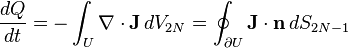
\frac{dQ}{dt}=- \int_U \nabla \cdot \mathbf{J} \, dV_{2N} = \oint_{\partial U} \mathbf{J} \cdot \mathbf{n} \, dS_{2N-1}

is the rate at which particles leave the hypersphere. (We take the sign convention from the well known case of continuity of charge or particles in three dimensions) Taking the limit that the length, L, of the hypercube vanishes, we have the 2N dimensional continuity equation,

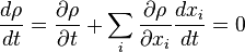
0= \frac{\partial\rho}{\partial t} + \nabla \cdot \mathbf{J}\;\mathrm{where}\;\nabla \cdot \mathbf{J}= \sum_{n=1}^{2N}\left(\frac{\partial(\rho\dot{q}_n)}{\partial q_n}+\frac{\partial(\rho\dot{p}_n)}{\partial p_n}\right)

The partial derivative reflects the fact that the hypercube remains stationary and does not move with the flow of particles in phase space. The divergence of the flow can be calculated as follows:

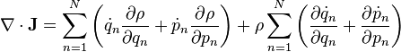
\nabla \cdot \mathbf{J}= \sum_{n=1}^{N}\left(\dot{q}_n\frac{\partial\rho}{\partial q_n} +\dot{p}_n\frac{\partial\rho}{\partial p_n}\right)+ \rho\sum_{n=1}^{N}\left(\frac{\partial\dot{q}_n}{\partial q_n} +\frac{\partial\dot{p}_n}{\partial p_n}\right)

The second term on the LHS vanishes because our variables obey Hamilton's equations of motion:

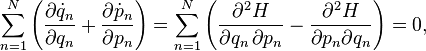
\sum_{n=1}^N\left( \frac{\partial\dot{q}_n}{\partial q_n} +\frac{\partial\dot{p}_n}{\partial p_n}\right) =\sum_{n=1}^N\left( \frac{\partial^2 H}{\partial q_n\,\partial p_n} -\frac{\partial^2 H}{\partial p_n \partial q_n}\right)=0,

The other term is a convective term of the form $\mathbf v\cdot\nabla\rho$ , where $\mathbf v = dx_i/dt$ . Liouville's equation is a statement about for the derivative of density in the reference frame of the points moving through phase space:

\frac{d\rho}{dt} = \frac{\partial\rho}{\partial t}+\sum_i \frac{\partial\rho}{\partial x_i}\frac{dx_i}{dt}=0

Never in the proof have we demanded that $\partial H/\partial t$ must vanish. Liouville's theorem is true even if the Hamiltonian is time dependent.

An alternative proof of Liouville's theorem is based on the time evolution of a volume element.^[8]^[9]

What Liouville's theorem does NOT imply

Liouville's theorem does not imply that the density is uniform throughout phase space. In particular, if the Hamiltonian preserves energy, then one trajectory cannot visit two parts of phase space with different energy. By the Boltzmann equation, if an ensemble has a property called 'temperature', then regions of phase space with more energy are less populated.
Liouville's theorem does not imply that every point along a given path has the same density. In other words, suppose that two particles, A and B, follow the same trajectory, except that particle A leads particle B by a finite time (or equivalently, there is a finite distance in xp space between the two particles). Particle A could be in a region of different density than particle B.
Liouville's theorem only holds in the limit that the particles are infinitely close together. Equivalently, Liouville's theorem does not hold for any ensemble that consists of a finite number of particles; instead the theorem describes the probability density in phase space of an ensemble consisting of an infinite number of possible states.

References and links

See also Introduction to entropy

↑ https://en.wikipedia.org/w/index.php?title=Perpetual_motion&oldid=584397707
↑ Jordan, T. "Steppingstones in Hamiltonian Dynamics", American Journal of Physics, Vol. 72, No. 8, pp. 1095-99, August 2004. States that theorem is valid if H depends on time. Proof uses divergence theorem in 2N dimensions.
↑ http://www.physics.purdue.edu/nlo/NoltePT10.pdf physics today
↑ https://www.math.okstate.edu/~binegar/4263/4263-l17.pdf states but never prove n dimensional divergence theorem
↑ https://en.wikipedia.org/wiki/Divergence_theorem#Multiple_dimensions
↑ http://hepweb.ucsd.edu/ph110b/110b_notes/node93.html
↑ http://www.lecture-notes.co.uk/susskind/classical-mechanics/lecture-7/liouvilles-theorem/ divergence theorem
↑ http://www.nyu.edu/classes/tuckerman/stat.mech/lectures/lecture_2/node2.html
↑ http://www.pma.caltech.edu/~mcc/Ph127/a/Lecture_3.pdf

This article is issued from Wikiversity - version of the Saturday, February 13, 2016. The text is available under the Creative Commons Attribution/Share Alike but additional terms may apply for the media files.