Strength of materials/Lesson 3
< Strength of materialsLesson 3: Stress transformation and Mohr's circle
Last time we talked about Hooke's law and plane stress. We also discussed how the normal and shear components of stress change depending on the orientation of the plane that they act on. In this lecture we will talk about stress transformations for plane stress.
For the rest of this lesson we assume that we are dealing only with plane stress,
i.e., there are only three nonzero stress components  ,
,  ,
,
 . We also assume that these three components are known.
We want to find the planes on which the stresses are most severe and the magnitudes of these stresses.
Stress transformation rules
Let us consider an arbitrary plane inside an infinitesimal element. Let this plane
be inclined at an angle  to the vertical face of the element. A free
body diagram of the region to the left of this plane is shown in the figure below.
to the vertical face of the element. A free
body diagram of the region to the left of this plane is shown in the figure below.
Stress transformation |
A balance of forces on the free body in the  -direction gives us

or,

Using the trigonometric identities

we get
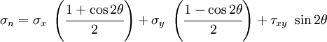
or,

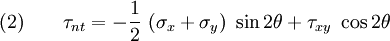
Similarly, a balance of forces in the  -direction leads to

or

or,
Now let us look at a section that is perpendicular to the one we have looked at. This situation is shown in the figure below.
Stress transformation |
In this case, a balance of forces on the free body in the -direction gives us

or,

or,
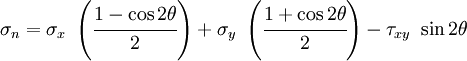
or,

A balance of forces in the -direction gives

or,

or,

From equations (2) and (4) we see that the shear stresses are equal. However the normal stresses on the two planes are different as you can see from equations (1) and (3).
You can think of the two cuts as just the faces of a new infinitesimal element
which is at an angle to the original element as can be seen form the
following figure.
Stress transformation |
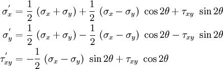
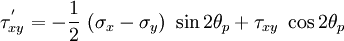
If we label the new normal stresses as  and
and  and the
shear stresses as
and the
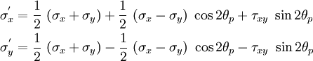
shear stresses as  , then we can write
Maximum normal stresses
What is the orientation of the infinitesimal element that produces the largest normal stress and the largest shear stress? This information can be useful in predicting where failure will occur.
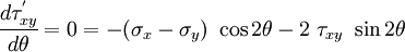
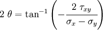
To find angle at which we get the maximum/minimum normal stress we can take the
derivatives of and with respect to and set them
to zero. So we have
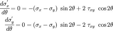
or,
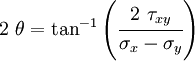
The angle at which is a maximum or a minimum is called a
principal angle or  .
.
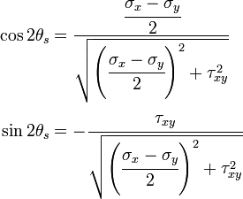
Now, from the identities
(or we can think in terms of a right angled triangle with a rise of
and a run of  )
)
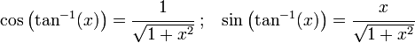
we have
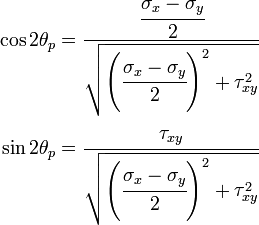
Taking another derivative with respect to we have
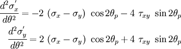
Plugging in the expressions for  and
and  we get
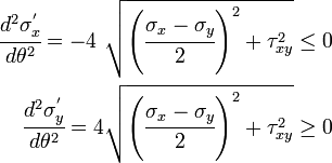
Clearly is a maximum while is a minimum value.
Principal stresses
The normal stresses corresponding to the principal angle are called the
principal stresses.
We have
Plugging in the expressions for and we get
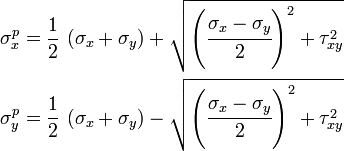
These principal stresses are often written as  and
and  or
or
 and
and  where
where  .
.
The value of the shear stress for an angle of is
Plugging in the expressions for and we get

Hence there are no shear stresses in the orientations where the stresses are maximum or minimum.
Maximum shear stresses
Similarly, we can find the value of which makes the shear stress a
maximum or minimum. Thus
or
In that case
The value of the shear stress for an angle of  is
is
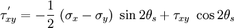
Plugging in the expressions for  and
and  we get
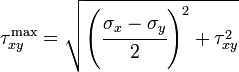
We can show that this is the maximum value of .
Note that, at the value of where is maximum, the normal stresses are not zero.
Mohr's circle
Mohr's idea was to express these algebraic relations in geometric form so that a physical interpretation of the idea became easier. The idea was based on the recognition that for an orientation equal to the principal angle, the stresses could be represented as the sides of a right-angled triangle.
Recall that
We can represent this in graphical form as shown in the figure below. In general, the locus of all points representing stresses at various orientations lie on a circle which is called Mohr's circle.
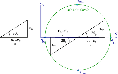 Mohr's circle |
Notice that we can directly find the largest normal stress and the small normal stress as well as the maximum shear stress directly from the circle. In three-dimensions there are two more Mohr's circles.
Negative shear stress
Also note that there is
a region where the shear stress  is negative. The convention that we
follow is that if the shear stress rotates the element clockwise then it is a
positive shear stress. If the element is rotated counter-clockwise then the
shear stress is negative.
is negative. The convention that we
follow is that if the shear stress rotates the element clockwise then it is a
positive shear stress. If the element is rotated counter-clockwise then the
shear stress is negative.
In the next lecture we will get into some more detail about actually plotting Mohr's circles.
External links
Professor Brannon's notes on Mohr's circle