Strength of materials/Lesson 2

Lesson 2: Elastic properties and plane stress

From the previous lesson you know that stress

is a point quantity.
has six components - three normal ( $\sigma$ ) and three shear ( $\tau$ ).
components depend on direction.
acts on a plane.
has units of force/area.

In this lesson we will introduce you to elastic properties and plane stress.

Elastic Properties

We will deal only with homogeneous and isotropic materials in this course. An isotropic material is one whose properties are independent of direction. Thus, if we want to do a test on a specimen of such a material, it does not matter from which part of the original material or in which direction we cut our sample out.

For an isotropic material we have to deal with three material properties of which only two are independent.

These material properties are

The Young's modulus ( $E$ ) (also called the modulus of elasticity).
The Poisson's ratio ( $\nu$ ).
The shear modulus ( $G$ ) (also called the modulus of rigidity).

Young's modulus ( $E$ )

Tension test

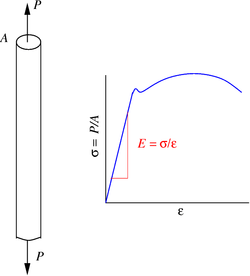
To find the Young's modulus we take a cylindrical specimen and pull on it uniaxially. The result is a stress-strain plot of the form shown in the adjacent figure.

The Young's modulus is defined as the ration of stress to strain in the linear elastic part of the stress-strain curve. Thus

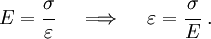
E = \cfrac{\sigma}{\varepsilon} \quad \implies \quad \varepsilon = \cfrac{\sigma}{E} ~.

Since the strain is dimensionless, the units of the Young's modulus are the same as the units of stress, i.e., force/area. In the English system, the units of the Young's modulus are psi while the SI units are Pa.

Representative values of Young's modulus are $10\times 10^6$ psi (10 Msi) or $70\times 10^9$ Pa (70 GPa) for aluminum and $29\times 10^6$ psi (29 Msi) or $200\times 10^9$ Pa (200 GPa) for steel. The higher the value of $E$ the stiffer a material. Note that stiffness and strength are two different concepts. Also, the value of Young's modulus does not vary much if the alloying content of a material is small compared to the amount of pure metal.

Poisson's ratio ( $\nu$ )

The Poisson's ratio is defined as

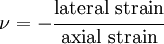
\nu = -\cfrac{\text{lateral strain}}{\text{axial strain}}

for an applied axial stress.

Poisson's ratio.

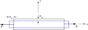
For the situation shown in the adjacent figure

\nu = - \cfrac{\varepsilon_y}{\varepsilon_x}

Values of Poisson's ratio range between 0.25 to 0.35 for most materials. Also, note that the shape of the cross section does not matter when we are measuring the Poisson's ratio as long as the applied stress is axial.

Shear modulus ( $G$ )

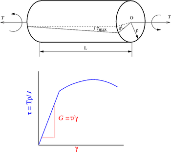Torsion test.

To find the shear modulus directly, we have to do a torsion test on a cylindrical specimen. A schematic of the stress-strain curve for such a test is shown in the adjacent figure.

The shear modulus is defined as

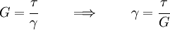
G = \cfrac{\tau}{\gamma} \qquad \implies \qquad \gamma = \cfrac{\tau}{G}

where $\tau$ is the shear stress and $\gamma$ is the shear strain.

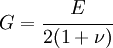
The shear modulus can be expressed in terms of $E$ and $\nu$ using the relation

G = \cfrac{E}{2(1+\nu)}

Hooke's law in three dimensions

The following table shows the strains that result when a stress is applied in a particular direction (or on a particular plane).

	Resulting strain
Applied stress	$\varepsilon_x$	$\varepsilon_y$	$\varepsilon_z$	$\gamma_{xy}\,$	$\gamma_{yz}\,$	$\gamma_{zx}\,$
$\sigma_x\,$	$\cfrac{\sigma_x}{E}$	$-\nu~\cfrac{\sigma_x}{E}$	$-\nu~\cfrac{\sigma_x}{E}$	0	0	0
$\sigma_y\,$	$-\nu~\cfrac{\sigma_y}{E}$	$\cfrac{\sigma_y}{E}$	$-\nu~\cfrac{\sigma_y}{E}$	0	0	0
$\sigma_z\,$	$-\nu~\cfrac{\sigma_z}{E}$	$-\nu~\cfrac{\sigma_z}{E}$	$\cfrac{\sigma_z}{E}$	0	0	0
$\tau_{xy}\,$	0	0	0	$\cfrac{\tau_{xy}}{G}$	0	0
$\tau_{yz}\,$	0	0	0	0	$\cfrac{\tau_{yz}}{G}$	0
$\tau_{zx}\,$	0	0	0	0	0	$\cfrac{\tau_{zx}}{G}$

You can check that these are indeed correct by looking at an infinitesimal element and seeing what the possible strains are when a particular stress component is applied.

Notice that normal stresses do not produce shear strains and shear stresses do not produce axial strains. This is only true for isotropic materials.

Principle of superposition

One of the advantages of working with linear elastic materials is that we can apply the principle of superposition. This principle states that the strains produced by a particular stress state $A$ can be added to those produced by a different stress state $B$ to get the strains for a combined stress state $A + B$ .

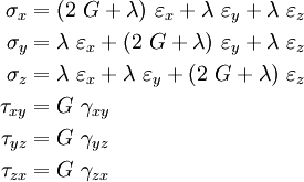
Applying the principle of superposition to the results in the table above, we find that if we have a stress state where all the stress components are active, then the strains are given by

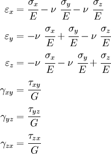
\begin{align} \varepsilon_x & = \cfrac{\sigma_x}{E}-\nu~\cfrac{\sigma_y}{E}-\nu~\cfrac{\sigma_z}{E} \\ \varepsilon_y & = -\nu~\cfrac{\sigma_x}{E}+\cfrac{\sigma_y}{E}-\nu~\cfrac{\sigma_z}{E}\\ \varepsilon_z & = -\nu~\cfrac{\sigma_x}{E}-\nu~\cfrac{\sigma_y}{E}+\cfrac{\sigma_z}{E}\\ \gamma_{xy} & = \cfrac{\tau_{xy}}{G} \\ \gamma_{yz} & = \cfrac{\tau_{yz}}{G} \\ \gamma_{zx} & = \cfrac{\tau_{zx}}{G} \end{align}

This relation is called the three-dimensional Hooke's law.

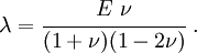
The inverse relation is

\begin{align} \sigma_x & = (2~G + \lambda)~\varepsilon_x + \lambda~\varepsilon_y + \lambda~\varepsilon_z \\ \sigma_y & = \lambda~\varepsilon_x + (2~G + \lambda)~\varepsilon_y + \lambda~\varepsilon_z \\ \sigma_z & = \lambda~\varepsilon_x + \lambda~\varepsilon_y + (2~G + \lambda)~\varepsilon_z \\ \tau_{xy} & = G~\gamma_{xy} \\ \tau_{yz} & = G~\gamma_{yz} \\ \tau_{zx} & = G~\gamma_{zx} \end{align}

where

\lambda = \cfrac{E~\nu}{(1+\nu)(1-2\nu)} ~.

Plane stress

It helps to think of plane stress as the state of stress on a plane with no stress!

Consider the infinitesimal cube shown in the adjacent figure. Assume that there is no stress on the plane perpendicular to the $z$ -axis. Then moment equilibrium requires that the out of plane shear stresses are also zero. In fact we can simplify the diagram and just draw a square instead of a cube as shown. But keep in mind that the shear stresses still act on a surface as do the normal stresses.

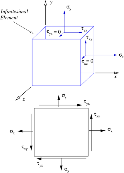Plane stress.

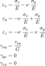
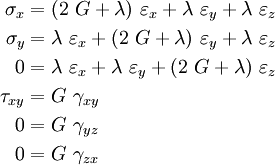
Therefore, in a state of plane stress, we have

\sigma_{z} = 0 ~;~~ \tau_{xz} = 0 ~;~~ \tau_{yz} = 0 ~.

For plane stress, Hooke's law takes the form

\begin{align} \varepsilon_x & = \cfrac{\sigma_x}{E}-\nu~\cfrac{\sigma_y}{E} \\ \varepsilon_y & = -\nu~\cfrac{\sigma_x}{E}+\cfrac{\sigma_y}{E} \\ \varepsilon_z & = -\nu~\cfrac{\sigma_x}{E}-\nu~\cfrac{\sigma_y}{E} \\ \gamma_{xy} & = \cfrac{\tau_{xy}}{G} \\ \gamma_{yz} & = 0 \\ \gamma_{zx} & = 0 \end{align}

Alternatively,

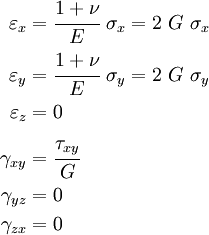
\begin{align} \sigma_x & = (2~G + \lambda)~\varepsilon_x + \lambda~\varepsilon_y + \lambda~\varepsilon_z \\ \sigma_y & = \lambda~\varepsilon_x + (2~G + \lambda)~\varepsilon_y + \lambda~\varepsilon_z \\ 0 & = \lambda~\varepsilon_x + \lambda~\varepsilon_y + (2~G + \lambda)~\varepsilon_z \\ \tau_{xy} & = G~\gamma_{xy} \\ 0 & = G~\gamma_{yz} \\ 0 & = G~\gamma_{zx} \end{align}

Effect of zero out of plane strain

Suppose, in addition, that $\varepsilon_z$ is also zero. What is the effect on Hooke's law?

We then have

\sigma_x = -\sigma_y

Therefore Hooke's law takes the form

\begin{align} \varepsilon_x & = \cfrac{1+\nu}{E}~\sigma_x = 2~G~\sigma_x \\ \varepsilon_y & = \cfrac{1+\nu}{E}~\sigma_y = 2~G~\sigma_y\\ \varepsilon_z & = 0 \\ \gamma_{xy} & = \cfrac{\tau_{xy}}{G} \\ \gamma_{yz} & = 0 \\ \gamma_{zx} & = 0 \end{align}

We will examine the significance of these relations in the next lesson.

This article is issued from Wikiversity - version of the Saturday, October 17, 2015. The text is available under the Creative Commons Attribution/Share Alike but additional terms may apply for the media files.