Heat equation/Solution to the 1-D Heat Equation

Definition

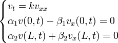
For the 1-dimensional case, the solution takes the form $u(x,t)$ since we are only concerned with one spatial direction and time. Thus the heat equation takes the form:

$u_t=ku_{xx}+h(x,t)$

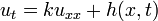
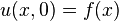
where k is our diffusivity constant and h(x,t) is the representation of internal heat sources. For our example, we impose the Robin boundary conditions, the initial condition, and the following bounds on our variables:

$(x,t)\in[0,L]\times[0,\infty)$
$u(x,0)=f(x)$
$\alpha_1u(0,t)-\beta_1u_x(0,t)=b_1(t)$
$\alpha_2u(L,t)+\beta_2u_x(L,t)=b_2(t)$
$\alpha_j,\beta_j \ge 0, \alpha_j^2+\beta_j^2 \ne 0$

Notice that the boundary conditions are non-homogeneous and time-dependent. The next few steps will illustrate one way to achieve a solution.

Solution

Step 1: Partition Solution

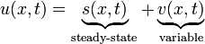
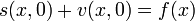
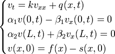
In order to get a solution, we can partition the function into a "transient" or "variable" solution and a "steady-state" solution:

$u(x,t)=\underbrace{s(x,t)}_{\text{steady-state}}+\underbrace{v(x,t)}_{\text{variable}}$

Substitute this relation into our original heat equation, boundary conditions and initial condition:

$s_t+v_t=ks_{xx}+kv_{xx}+h(x,t)$
$\alpha_1s(0,t)+\alpha_1v(0,t)-\beta_1s_x(0,t)-\beta_1v_x(0,t)=b_1(t)$
$\alpha_2s(L,t)+\alpha_2v(L,t)+\beta_2s_x(L,t)+\beta_2v_x(L,t)=b_2(t)$
$s(x,0)+v(x,0)=f(x)$

We will also impose conditions on our partitioned solutions. Part of the beauty of partitioning the solution is being able to divide the boundary conditions among both parts. The following conditions will be imposed:

We will choose the steady-state solution to be linear in x, which means that $s_{xx}=0~.$
We will let the steady-state solution handle the non-homogeneous boundary conditions.
We will let the variable portion satisfy the non-homogeneous equation and homogeneous boundary conditions.

Thus, we have constructed two separate initial boundary value problems (IBVPs):

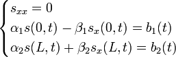
$\begin{cases} s_{xx} = 0 \\ \alpha_1s(0,t)-\beta_1s_x(0,t)=b_1(t) \\ \alpha_2s(L,t)+\beta_2s_x(L,t)=b_2(t) \end{cases}$

$\begin{cases} v_t=kv_{xx}-s_t+h(x,t) \\ \alpha_1v(0,t)-\beta_1v_x(0,t)=0\\ \alpha_2v(L,t)+\beta_2v_x(L,t)=0\\ v(x,0)=f(x)-s(x,0) \end{cases}$

Note that the sum $s(x,t)+v(x,t)$ satisfies all conditions of the original IBVP.

Step 2: Solve Steady-state Partition

Assumption 1

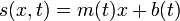
We are assuming that S is linear in x, so our equation take the form:

$s(x,t)=m(t)x+b(t)$

We will see why this is only an assumption because doesn't cover all the different boundary condition types. Applying the boundary conditions, we get:

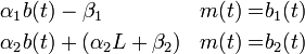
$\begin{align} \alpha_1 & b(t)-\beta_1 & m(t) = & b_1(t) \\ \alpha_2 & b(t)+(\alpha_2 L+\beta_2) & m(t) = & b_2(t) \end{align}$

Solving for $b(t)$ and $m(t)$ :

$b(t)=\frac{\begin{vmatrix} b_1(t) & -\beta_1 \\ b_2(t) & \alpha_2 L+\beta_2 \end{vmatrix} }{\begin{vmatrix} \alpha_1 & -\beta_1 \\ \alpha_2 & \alpha_2 L+\beta_2 \end{vmatrix} }=\frac{(\alpha_2 L+\beta_2)b_1(t)+\beta_1b_2(t)}{\alpha_1\alpha_2L+\alpha_1\beta_2+\alpha_2\beta_1}$
$m(t)=\frac{\begin{vmatrix} \alpha_1 & b_1(t) \\ \alpha_2 & b_2(t) \end{vmatrix} }{\begin{vmatrix} \alpha_1 & -\beta_1 \\ \alpha_2 & \alpha_2 L+\beta_2 \end{vmatrix} }=\frac{\alpha_1b_2(t)-\alpha_2b_1(t)}{\alpha_1\alpha_2L+\alpha_1\beta_2+\alpha_2\beta_1}$
$s(x,t)=\frac{\alpha_1b_2(t)-\alpha_2b_1(t)}{\alpha_1\alpha_2L+\alpha_1\beta_2+\alpha_2\beta_1} x + \frac{(\alpha_2 L+\beta_2)b_1(t)+\beta_1b_2(t)}{\alpha_1\alpha_2L+\alpha_1\beta_2+\alpha_2\beta_1}$

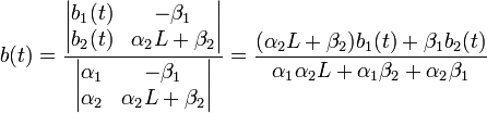
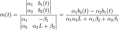
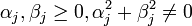
That means that the coefficients are only defined as long as $\alpha_1\alpha_2L+\alpha_1\beta_2+\alpha_2\beta_1 \ne 0~.$ This means that the linear assumption of s(x,t) only holds if the boundary conditions are not both Neumann type (i.e. $\alpha_1,\alpha_2 \ne 0$ ). Knowing the coefficients $\alpha_1,\alpha_2,\beta_1,\beta_2$ from the original boundary conditions will yield the coefficients for s(x,t).

Assumption 2

For the case where both boundary conditions are Neumann type, a different assumption must be made. The linear assumption didn't yield any solution, so let's assume s has a quadratic relationship with x:

$s(x,t)=a(t)x^2+b(t)x+c(t)~.$

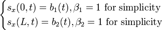
For convenience, we choose $c(t)=0~.$ In this Neumann-Neumann condition, the only boundary conditions we have are:

$\begin{cases} s_x(0,t)=b_1(t), \beta_1=1 \text{ for simplicity}\\ s_x(L,t)=b_2(t), \beta_2=1 \text{ for simplicity} \end{cases}$

Solving the assumption for the boundary conditions:

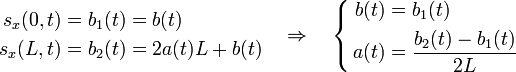
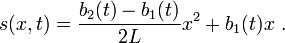
$\begin{align} s_x(0,t)&=b_1(t)=b(t) \\ s_x(L,t)&=b_2(t)=2a(t)L+b(t) \end{align} \quad \Rightarrow \quad \left \{ \begin{align} b(t)&=b_1(t)\\ a(t)&=\frac{b_2(t)-b_1(t)}{2L} \end{align} \right .$

Thus we arrive at the solution to the "steady-state" solution:

$s(x,t)=\frac{b_2(t)-b_1(t)}{2L} x^2 + b_1(t) x~.$

Step 3: Solve Variable Partition

The equation for the variable portion is:

$v_t=kv_{xx}-s_t+h(x,t)+ks_{xx}$

For Assumption 1

In order to simplify the equation, we can define a new function:

$q(x,t):=h(x,t)-s_t(x,t)$

For Assumption 2

In order to simplify the equation, we can define a new function:

$q(x,t):=h(x,t)-s_t(x,t)+ks_{xx}(x,t)$

Step 3.1: Solve the Associated Homogeneous IBVP

The associated homogeneous IBVP is as follows:

$\begin{cases} v_t=kv_{xx} \\ \alpha_1v(0,t)-\beta_1v_x(0,t)=0 \\ \alpha_2v(L,t)+\beta_2v_x(L,t)=0 \end{cases}$

Separate Variables

$v(x,t)=X(x)T(t) \Rightarrow XT'=kX''T \Rightarrow \frac{T'}{kT} = \frac{X''}{X} = \mu$

Translate Boundary Conditions

$\begin{align} 0 & = \alpha_1X(0)T(t)-\beta_1X'(0)T(t) & \\ & = \left [ \alpha_1X(0)-\beta_1X'(0) \right ]T(t) & \forall t \in [0,\infty) \\ \end{align} \quad \Rightarrow \quad \alpha_1X(0)-\beta_1X'(0)=0$

$\begin{align} 0 & = \alpha_2X(L)T(t)+\beta_2X'(L)T(t) & \\ & = \left [ \alpha_2X(L)+\beta_2X'(L) \right ]T(t) & \forall t \in [0,\infty) \\ \end{align} \quad \Rightarrow \quad \alpha_2X(L)+\beta_2X'(L)=0$

Solve the SLP

$\left . \begin{align} X''-\mu X = 0\\ \alpha_1X(0)-\beta_1X'(0)=0 \\ \alpha_2X(L)+\beta_2X'(L)=0 \end{align} \right \} \begin{align} -\mu & = \lambda^2 \\ \lambda_n & =\text{ solutions to equation } (\alpha_1\alpha_2-\beta_1\beta_2\lambda^2)\sin (\lambda L)+(\alpha_1\beta_2+\alpha_2\beta_1)\lambda \cos (\lambda L) = 0 \\ X_n(x) & =\beta_1\lambda_n \cos (\lambda_n x) + \alpha_1 \sin(\lambda_n x) \end{align}$

Step 3.2: Solve the Non-homogeneous BVP

The BVP is as follows:

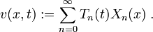
$\begin{cases} v_t=kv_{xx}+q(x,t) \\ \alpha_1v(0,t)-\beta_1v_x(0,t)=0 \\ \alpha_2v(L,t)+\beta_2v_x(L,t)=0 \\ v(x,0)=f(x)-s(x,0) \end{cases}$

In order to solve the problem, let:

$v(x,t):=\sum_{n=0}^\infty T_n(t)X_n(x)$

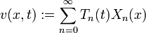
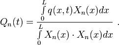
where the time-dependent Fourier coefficients will be determined later. Also, let:

$q(x,t):=\sum_{n=0}^\infty Q_n(t)X_n(x)$

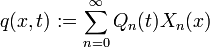
where the Fourier coefficients are given by the inner product:

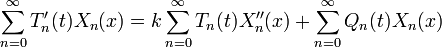
$Q_n(t)=\frac{\int\limits_0^L q(x,t)X_n(x) dx}{\int\limits_0^L X_n(x) \cdot X_n(x) dx}~.$

In order to solve for the coefficients $T_n(t)$ , we have to substitute the relations above into the original PDE. The term-by-term differentiation of v is legitimate since the partial derivatives of v are continuous. v satisfies the same spatial boundary conditions as the eigenfunction:

$\frac{\partial}{\partial t} \left [ \sum_{n=0}^\infty T_n(t)X_n(x) \right ] = k \frac{\partial^2}{\partial x^2} \left [ \sum_{n=0}^\infty T_n(t)X_n(x) \right ] + \sum_{n=0}^\infty Q_n(t)X_n(x)$
$\sum_{n=0}^\infty T_n'(t)X_n(x) = k \sum_{n=0}^\infty T_n(t)X_n''(x) + \sum_{n=0}^\infty Q_n(t)X_n(x)$

Since the eigenfunction $X_n(x)$ satisfies the ODE $X''+\lambda_n^2 X=0 \Rightarrow X_n''(x)=-\lambda_n^2 X_n(x)$ ,

$\sum_{n=0}^\infty T_n'(t)X_n(x) = \sum_{n=0}^\infty -k\lambda_n^2T_n(t)X_n(x) + \sum_{n=0}^\infty Q_n(t)X_n(x)$
$\sum_{n=0}^\infty \left [ T_n'(t)+k\lambda_n^2T_n(t) \right ] X_n(x) = \sum_{n=0}^\infty Q_n(t)X_n(x)$

Since $X_n(x)$ forms a basis and is therefore linearly independent:

$T_n'(t)+k\lambda_n^2T_n(t)=Q_n(t)$

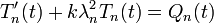
which is a first order non-homogeneous linear equation. The integrating factor 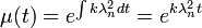$\mu(t)=e^{\int k\lambda_n^2 dt}=e^{k\lambda_n^2t}$ . Solving the equation yields:

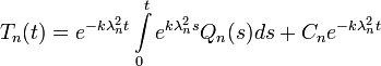
$T_n(t)=e^{-k\lambda_n^2t} \int\limits_0^t e^{k\lambda_n^2s}Q_n(s) ds + C_ne^{-k\lambda_n^2t}$

The constant $C_n$ allows us to satisfy the initial condition:

$v(x,0)=f(x)-s(x,0)=\sum_{n=0}^\infty T_n(0)X_n(x)=\sum_{n=0}^\infty C_nX_n(x)~.$
$C_n=\frac{\int\limits_0^L \left [ f(x)-s(x,0) \right ] X_n(x) dx}{\int\limits_0^L X_n(x) \cdot X_n(x) dx}~.$

We can now substitute all the expressions to get the variable portion $v(x,t)$ :

Compute and substitute $C_n$ and $Q_n(t)$ into $T_n(t)~.$
Compute and substitute $T_n(t)$ and $X_n(x)$ into $v(x,t):=\sum_{n=0}^\infty T_n(t)X_n(x)~.$

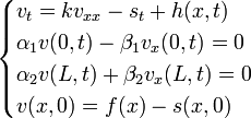
Step 4: Combine Solutions

The complete solution for $u(x,t)$ can be found by adding the "steady-state" solution and the "variable" solutions. The result can easily be checked by graphing in a symbolic solver like Mathematica or Maple.

This article is issued from Wikiversity - version of the Saturday, July 09, 2011. The text is available under the Creative Commons Attribution/Share Alike but additional terms may apply for the media files.