Shifted inverse iteration

We can apply the w:power method to find the largest eigenvalue and the w:inverse power method to find the smallest eigenvalue of a given matrix.We can also find the middle eigenvalue by the shifted inverse power method. Before explaining this method, I'd like to introduce some theorems which are very necessary to understand it.

Background Theorems

(See http://www.math.nuk.edu.tw/jinnliu/Software_Engineering/IS_PowerMethod.pdf)

Suppose that λ and a nonzero vector V are an eigenpair of A. If α is any constant, then λ- α and V are an eigenpair of the matrix  $(A - \alpha I)$ .

Suppose that λ and a nonzero vector V are an eigenpair of A. If  λ is not equal to α, then 1/(λ -α) and V are an eigenpair of the matrix  $(A - \alpha I)^{-1}$ .

Shifted inverse power method

Assume that the n×n matrix A has distinct w:eigenvalues $\lambda_1$ , $\lambda_2$ ,.... $\lambda_n$ and consider the eigenvalue $\lambda_j$ . Then a constant α can be chosen so that

\sigma_1

=1 / (

\lambda_j

- α)

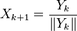
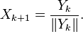
is the dominant eigenvalue of $(A - \alpha I)^{-1}$ . Furthermore, if $X_0$ is chosen appropriately which is the initial guess vector, then the sequences $\left( X_{k} \right)$ defined by

Y_k=(A - \alpha I)^{-1}X_k

X_{k+1} = \frac{Y_k}{\|Y_k\|}

and $\left( c_{k} \right)$ defined by

c_k = \frac{Y_k^\top X_k}{X_k^\top X_k}

(w:Rayleigh quotient)

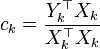will converge to the dominant eigenpair $\sigma_1$ , $V_j$ of the matrix $(A - \alpha I)^{-1}$ . Therefore, the corresponding eigenvalue for the matrix A is given by

\lambda_j= 1 /\sigma_1 + \alpha

Example

Use the shifted inverse power method to find the eigenpairs of the matrix

$A=\left[\begin{array}{c c c}0 & 11 & -5 \\-2 & 17 & -7 \\-4 & 26 & -10 \end{array} \right]$ .

Use the fact that the eigenvalues of A are $\lambda_1$ =4, $\lambda_2$ =2, $\lambda_3$ =1, and select an appropriate α and starting vector for each case.

Case1: For the eigenvalue $\lambda_1$ =4, we select α=4.2 and the starting vector

$X_0=\left[\begin{array}{c}1 \\1 \\ 1 \\\end{array} \right]$ .

First we can get

$(A - 4.2 I)= \left[\begin{array}{c c c}-4.2 & 11 & -5 \\-2 & 12.8 & -7 \\-4 & 26 & -14.2 \end{array} \right]$

and then we can apply the shifted inverse power method

$Y_k$ = $(A - \alpha I)^{-1}$ $X_k$ .

Therefore,

$\left[\begin{array}{c c c}-4.2 & 11 & -5 \\-2 & 12.8 & -7 \\-4 & 26 & -14.2 \end{array} \right]$ $Y_0$ = $X_0=\left[\begin{array}{c}1 \\1 \\ 1 \\\end{array} \right]$ .

Solving this system of equations, we get

$Y_0=\left[\begin{array}{c}-9.545454545 \\-14.09090909 \\ -23.18181818 \\\end{array} \right]$ .

Next we can compute

$c_1$ = $\frac{Y_0^\top X_0}{X_0^\top X_0}.$ ,

so $c_1$ =-15.606060605. Since

$X_{k+1} = \frac{Y_k}{\|Y_k\|}.$ ,

it implies

$X_1=\left[\begin{array}{c}-0.4117 \\-0.6078 \\ -1 \\\end{array} \right]$ .

We continue doing the second iteration:

$\left[\begin{array}{c c c}-4.2 & 11 & -5 \\-2 & 12.8 & -7 \\-4 & 26 & -14.2 \end{array} \right]$ $Y_1$ = $X_1=\left[\begin{array}{c}-0.4117 \\-0.6078 \\ -1 \\\end{array} \right]$ .

Thus

$Y_1=\left[\begin{array}{c}2.14795 \\3.21746 \\ 5.35650 \\\end{array} \right]$ .

It implies $c_2$ =-5.326069 and

$X_2=\left[\begin{array}{c}0.400998 \\0.600665 \\ 1 \\\end{array} \right]$ .

We should continue the iteration and finally we got the sequence $\left( c_{k} \right)$ will converge to $\sigma_1=-5$ , which is the dominant eigenvalue of $(A - 4.2 I)^{-1}$ , and the sequences $\left( X_{k} \right)$ converges to

$V_1=\left[\begin{array}{c}0.4 \\0.6 \\ 1 \\\end{array} \right]$

after 9 iterations. We can get the eigenvalue $\lambda_1$ of A by the formula:

$\lambda_1$ = 1 / $\sigma_1$ + α= 1/(-5) + 4.2 =4.

We can apply the same approach to find another two eigenvalues of the given matrix A.

Exercise

Use the shifted inverse power method to find the eigenvalue

$\lambda_2$ =2

for the same matrix A as the example above, given the starting vector

$X_0=\left[\begin{array}{c}1 \\1 \\ 1 \\\end{array} \right]$ ,

α=2.1.

Solution:

For the eigenvalue

$\lambda_1$ =2,

we select α=2.1 and the starting vector

$X_0=\left[\begin{array}{c}1 \\1 \\ 1 \\\end{array} \right]$ .

First we can get

$(A - 2.1 I)= \left[\begin{array}{c c c}-2.1 & 11 & -5 \\-2 & 14.9 & -7 \\-4 & 26 & -12.1 \end{array} \right]$ .

Therefore,

$\left[\begin{array}{c c c}-2.1 & 11 & -5 \\-2 & 14.9 & -7 \\-4 & 26 & -12.1 \end{array} \right]$ $Y_0$ = $X_0=\left[\begin{array}{c}1 \\1 \\ 1 \\\end{array} \right]$ .

$Y_0=\left[\begin{array}{c}11.05263158 \\21.57894737 \\ 42.63157895 \\\end{array} \right]$

and

$c_1=25.0877193$

It implies

$X_1=\left[\begin{array}{c}0.2592592593 \\0.5061728395 \\ 1 \\\end{array} \right]$ .

After 7 iterations,we got

$\sigma_1=-10$

and

$V_1=\left[\begin{array}{c}0.25 \\0.5 \\ 1 \\\end{array} \right]$ .

Doing some computation, We got

$\lambda_1$ = 1 / $\sigma_1$ + α= 1/(-10) + 2.1 =2.

Exercise

Use w:Matlab to do the shifted inverse power method to find the eigenvalue $\lambda_2$ =5.1433 for the given matrix

$A=\left[\begin{array}{c c c}6 &2 & -1 \\2 & 5 & 1 \\-1 & 1 & 4 \end{array} \right]$ .

The starting vector is

$X_0=\left[\begin{array}{c}1 \\1 \\ 3 \\\end{array} \right]$ ,

α=6.

Solution:

First we can get

$(A - 6 I)= \left[\begin{array}{c c c}0 & 2 & -1 \\2 & -1 & 1 \\-1 & 1 & -2 \end{array} \right]$ .

Then we can apply the method mentioned above to find the middle eigenvalue of the matrix. Below is the Matlab code for this question.

for i=1:7
    y=linsolve(A,x);
    e=(y'*x)/(x'*x);
    x=y/norm(y);
end

We can find that the sequence $\left( c_{k} \right)$ will converge to $\sigma_2=-1.167238857441354$ after 7 iterations. Doing some computation, We got

$\lambda_2$ = 1 / $\sigma_2$ + α= 1/(-1.167238857441354) + 6 = 5.143277321839636

which is approximately equal to 5.1433, the middle eigenvalue of the matrix.

Reference

Yu-Kai Hong,An introduction to the Power Method and (shifted/Inverse) Power Method,2007

John H.Mathews,Kurtis D.Fink,Numerical method using Matlab,4th edition,2004

This article is issued from Wikiversity - version of the Tuesday, December 11, 2012. The text is available under the Creative Commons Attribution/Share Alike but additional terms may apply for the media files.