Physics/Essays/Fedosin/Selfconsistent electromagnetic constants
< Physics < Essays < FedosinSelfconsistent electromagnetic constants is the full set of fundamental constants of classical electromagnetism that are selfconsistent and determine the external definitions of different physical quantities (and its fundamental dimensions), and therefore – the resulting set of the Maxwell's equations. The constants are confirmed by the fact that they work in any systems of measurement and are part of vacuum constants.
The primary set of electromagnetic constants is:
- the first electromagnetic constant (
 ), which is the speed of light or speed of the electromagnetic waves in free space;
  metres per second.[1]
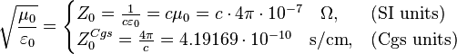
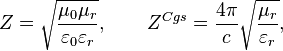
 - the second electromagnetic constant, which is the impedance of free space
 Ω.[2]
Ω.[2]
The secondary set of electromagnetic constants is:
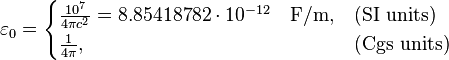
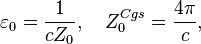
1. the electric constant or vacuum permittivity:
2. the magnetic constant or vacuum permeability:
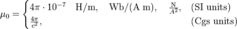
Both, primary and secondary sets of electromagnetic constants are selfconsistent, because they are connected by the following relations:

Note that in the Cgs units  and
and  are in the "latent form" and therefore are not defined evidently, but they are the same as defined above.
Furthermore, the values of impedance of free space in the SI units and Cgs units are connected by the following relation: [3]
are in the "latent form" and therefore are not defined evidently, but they are the same as defined above.
Furthermore, the values of impedance of free space in the SI units and Cgs units are connected by the following relation: [3]

Connection with other constants
The electromagnetic constants may be found in many equations and also connect with other constants. Introducing the Planck constant  and the elementary charge
  we find:
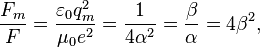
the fine structure constant  ,
,
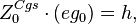
the von Klitzing constant  ,
,
the impedance of free space  .
.
Another example is the strong gravitational constant 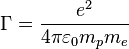 ,
,
where  – the mass of proton,
  – the mass of electron.
History
There is the delicate problem of electromagnetic constants in the classical electromagnetism up to now. Actually, in the CGS units only two constants:
 (speed of light) and
  are used,[4]
but in the SI units there are four constants:
are used,[4]
but in the SI units there are four constants:
 (vacuum permittivity),
 (vacuum permeability),
( speed of light) and (impedance of free space).
Furthermore, the impedance of free space was introduced by Stratton only in the 1941,[5]
which are widely used in the applied physics. But the second set ( and ) is mostly considered as "artificial" ones, that have no physical meaning,[6] and used only for the sake of dimension consistency of the physical quantities (such as in electrostatic induction with , and in electromagnetic induction with ).
(vacuum permeability),
( speed of light) and (impedance of free space).
Furthermore, the impedance of free space was introduced by Stratton only in the 1941,[5]
which are widely used in the applied physics. But the second set ( and ) is mostly considered as "artificial" ones, that have no physical meaning,[6] and used only for the sake of dimension consistency of the physical quantities (such as in electrostatic induction with , and in electromagnetic induction with ).
However, with the discovery of the w:Quantum Hall effect by von Klitzing (1981)[7] the theorists paid serious attention to the physical essence of resistance (or impedance), which is due to the charges or fluxes. Actually, Yakymakha (1989)[8] first introduced the magnetic coupling constant, defined through the magnetic monopole,[9] and in the 1994[10] for the first time the impedance of free space was observed in the quantum 2D-electron system at the silicon- dioxide interface of the serial MOSFETs. Further, Tsu and Datta (2003)[11][12] considered for the first time the new interpretation of the wave function in the Schrodinger equation, defined through the impedance of free space. Increasing attention to the impedance of free space as part of the general problem of the characteristic impedance was shown by Zel’dovich (2008).<ref name =Zel'dovich1> Zel'dovich, B.Y.` (2008). "Impedance and parametric excitation of oscillators". UFN 178 (5). http://www.mathnet.ru/php/archive.phtml?wshow=paper&jrnid=ufn&paperid=596&option_lang=rus.</ref>
Application
Electromagnetic fields
The main conception of the Cgs units is defined on the primary nature of electromagnetic fields. So, here we have the same dimensions for electric and magnetic fields:
![[E] = [D] = [H] = [B] = L^{-1/2}M^{1/2}T^{-1} \](../I/m/b8e81fc8692efeface88222c086f7473.png)
Contrary to the Cgs units, the SI units have different dimensions of the electromagnetic fields (in vacuum):


which is based on the different dimensions of electric and magnetic charges:
![[e]^{SI} = \](../I/m/e2034c0819148f99edc0964183801253.png) Coulomb,
Coulomb,![[q_m]^{SI} = \](../I/m/2083f7f9b52dd714a473953aa5fb57f4.png) J/A.
J/A.
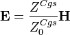
In the general case, when the space is filled by matter, these definitions are changed:


where  is the relative permittivity, and
  is the relative permeability.
In the electromagnetic wave propagation process we have the following relationships between electric and magnetic fields:
 (Cgs units)
 (SI units)
Note that, in the Cgs units it is hard to define the wave impedance, and therefore it is often said that there are no any wave impedance.[13] But using the generalized definition of the wave impedance in the form:
we can rewrite the above equations for the wave in the general form:
 (Cgs units)
 (SI units)
where the fact of the same dimensions of electric and magnetic fields in the Cgs units is considered.
Reactive parameters
The same problem of dimensions equality is presented in the Cgs units for reactive parameters. Actually, the standard capacitance is defined as:

where the dimension of electric charge in Cgs units is ![[Q] = L^{3/2}M^{1/2}T^{-1} \](../I/m/d92ec1e57f53426645d5de19aa2faeb7.png) , and the dimension of electric voltage is
, and the dimension of electric voltage is ![[V] = L^{1/2}M^{1/2}T^{-1} \](../I/m/a0788ebde2eca5a34e8fd339a7158603.png) . So, capacitance in the Cgs units has dimension of the length
. So, capacitance in the Cgs units has dimension of the length ![[C] = L. \](../I/m/11082d0afa1e87002420ac1bdb12e011.png) Furthermore, the standard inductance is defined as:
Furthermore, the standard inductance is defined as:

where the dimension of magnetic flux is ![[\Phi] = L^{3/2}M^{1/2}T^{-1} \](../I/m/18d15b77ef06b4c8af8baef4409213fa.png) , and the dimension of electric current in the Cgs units is
, and the dimension of electric current in the Cgs units is ![[I] = L^{3/2}M^{1/2}T^{-2} \](../I/m/1e0eda602564f30b14e6e2c37297cff4.png) . So, inductance has the same dimension of the length
. So, inductance has the same dimension of the length ![[L] = L \](../I/m/cb9937ed952542c3c5120df0055b535d.png) .
.
LC circuit
The main problem in the Cgs units is the LC circuit resonance parameters. Actually, the natural values of the resonance frequency ( ) and characteristic impedance (
 ) in a lossless line are working well in the SI units only:


But in the Cgs units characteristic impedance is dimensionless and angular frequency is reverse square of the length. Therefore, theoretics which prefer Cgs units, when considering LC circuit use the SI units.[4] So, redefinition of them through the electromagnetic constants is needed:


Maxwell equations
Considering the following relationships between electromagnetic constants:

In the Cgs units, macroscopic Maxwell's equations can be rewritten in the normalized form:
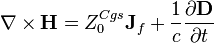
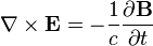

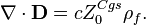
where  is the free electric charge 3D-density, and
  is the current density of free charges.
Note that in this normalized form there are only the primary electromagnetic constants included (without ).
Coulomb force
The electric Coulomb's Law for two elementary charges  is defined as:
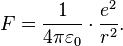
In the Cgs units we have:

The magnetic force between two fictitious elementary magnetic charges can be defined as follows:
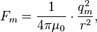
where  is the magnetic charge.
The same in the Cgs units is:
is the magnetic charge.
The same in the Cgs units is:

where
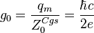
is the normalized magnetic charge (or Dirac's monopole in the Cgs units). [14][15] Furthermore, electric and magnetic charges in the Cgs units have the same dimensions:
![[g_0] = [e] = L^{3/2}M^{1/2}T^{-1} \](../I/m/ec698571f9e86bfb40db368139d660c8.png)
and could be compared:
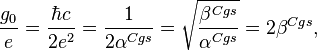
where  is the electric fine structure constant in the Cgs units, and
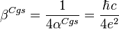 is the magnetic coupling constant in the Cgs units for the fictitious magnetic charges.
Thus, the relationship between Coulomb forces will be:
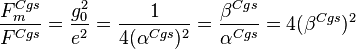
which is the same as in the SI units:
where 
Quanta of action
In consistence to the Quantum Electromagnetic Resonator approach, the charge multiplication (electric and magnetic) should be equal to the quant of action:

where is the electric charge,  is the magnetic charge, and
  is the Planck constant (or the quant of action).
There are no problems in the SI units, where  , but in the Cgs units we have the same dimensions of the charges:
![[e] = [g_0]. \](../I/m/123b7a0546fd08f81df87e121fb53471.png)
Therefore, to restore the self consistence of the Cgs units we should to consider the second electromagnetic constant  :
:
which is an analog of the uncertainty principle in the quantum mechanics.
Quantum Hall effect
Simple theory presented by Laughlin[16] to explain QHE [7] used the following definition of the adiabatic strip current in the Cgs units:
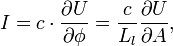
where  is the magnetic flux,
  is the vector potential, and
  is the strip length.
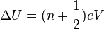
Using the following changes of total energy
is the strip length.
Using the following changes of total energy  and magnetic flux between Landau levels:
we obtain the following current:
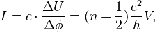
where  , and
, and  is effective potential of the level. Note that, this magnetic flux quantum
 is different from Dirac monopole:

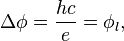
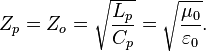
Photon as quantum resonator
Let us consider  and
and  as quantum capacitance and inductance of free photon in the SI units. We shall suppose that characteristic impedance of photon equals to the impedance of free space:
Then the resonance frequency will be:
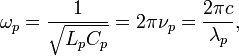
where  is wavelength of photon.
The solution of these two equations will be:
is wavelength of photon.
The solution of these two equations will be:
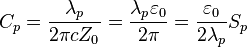
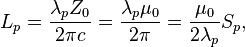
where 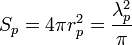 and
and
 is the photon intrinsic radius.
See also
- International System of Units
- Centimetre–gram–second system of units
- Classical electromagnetism
- Quantum Electromagnetic Resonator
- Selfconsistent gravitational constants
Notes
- ↑ "CODATA value: Speed of Light in Vacuum". The NIST reference on Constants, Units, and Uncertainty. NIST. Retrieved 2009-08-21.
- ↑ "Characteristic impedance of vacuum, Z0". The NIST reference on constants, units, and uncertainty: Fundamental physical constants. NIST. Retrieved 2011-11-28.
- ↑ Бредов М.М., Румянцев В.В., Топтыгин И.Н. (1985). "Appendix 5: Units transform (p.385)". Классическая электродинамика. Nauka.
- ↑ 4.0 4.1 amm I.E. (1989). Основы теории электричества. Moscow: Nauka. ISBN 5-02-014244-1.
- ↑ Stratton J.A. (1941). Electromagnetic Theory. New York, London: McGraw-Hill. http://lib.org.by/info/P_Physics/PE_Electromagnetism/Stratton%20J.A.%20Electromagnetic%20Theory%20(MGH,%201941)(T)(631s)_PE_.djvu.
- ↑ Кузьмичев В.Е. (1989). Законы и формулы физики. Kiev: Naukova Dumka. ISBN 5-12-000493-8.
- ↑ 7.0 7.1 von Klitzing, K.; Dorda, G.; Pepper, M. (1980). "New Method for High-Accuracy Determination of the Fine-Structure Constant Based on Quantized Hall Resistance". Physical Review Letters 45 (6): 494–497. doi:10.1103/PhysRevLett.45.494.
- ↑ Yakymakha O.L.(1989). High Temperature Quantum Galvanomagnetic Effects in the Two- Dimensional Inversion Layers of MOSFET's (In Russian). Kiev: Vyscha Shkola. p.91. ISBN 5-11-002309-3. djvu
- ↑ Dirac P.A.M., Proc.Roy.Soc. (London), Ser. A,133, 60 (1931)
- ↑ Yakymakha O.L., Kalnibolotskij Y.M. (1994). "Very-low-frequency resonance of MOSFET amplifier parameters". Solid- State Electronics 37(10),1739-1751 Pdf
- ↑ Timir Datta; Raphael Tsu (2003). "Quantum Wave Resistance of Schrodinger functions". arXiv:cond-mat/0311479 [cond-mat].
- ↑ Raphael Tsu and Timir Datta (2008) “Conductance and Wave Impedance of Electrons”. Progress In Electromagnetics Research Symposium, Hangzhou, China, March 24-28 Pdf
- ↑ Сена Л.А. (1988). Единицы физических величин и их размерности (3-е изд.). Moscow: Nauka. ISBN 5-02-013848-7.
- ↑ Schwinger, J. (1969). "A magnetic model of matter". Science 165 (3895): 757.
- ↑ Devons, S. (1963). "Search for magnetic monopole". Sci. Progr. 51 (204): 601.
- ↑ Laughlin, R. B. (1981). "Quantized Hall conductivity in two dimensions". Phys. Rev. B. 23 (10): 5632–5633. doi:10.1103/PhysRevB.23.5632.
References
- Hallock, William; Wade, Herbert Treadwell (1906). Outlines of the evolution of weights and measures and the metric system. New York: The Macmillan Co. p. 200. http://books.google.com/books?id=NVZKAAAAMAAJ.
- Griffiths, David J. (1999). "Appendix C: Units". Introduction to Electrodynamics (3rd ed.). Prentice Hall. ISBN 0-13-805326-X.
- Jackson, John D. (1999). "Appendix on Units and Dimensions". Classical Electrodynamics (3rd ed.). Wiley. ISBN 0-471-30932-X.
- Littlejohn, Robert (Fall 2007). "Gaussian, SI and Other Systems of Units in Electromagnetic Theory" (pdf). Physics 221A, University of California, Berkeley lecture notes. Retrieved 2008-05-06.
- Stratton J.A. (1941). Electromagnetic Theory. New York, London: McGraw-Hill. http://lib.org.by/info/P_Physics/PE_Electromagnetism/Stratton%20J.A.%20Electromagnetic%20Theory%20(MGH,%201941)(T)(631s)_PE_.djvu.
- Детлаф А.А., Яворский Б.М., Милковская Л.Б. (1977). "Reference Book on Electricity" djvu Курс физики. Том 2. Электричество и магнетизм (4-е издание). Moscow: Vysshaya Shkola. http://eqworld.ipmnet.ru/ru/library/books/DetlafYavorskijMilkovskaya_t2_1977ru.djvu "Reference Book on Electricity" djvu.
- Гольдштейн Л.Д., Зернов Н.В. (1971). "Electromagnetic Fields" Электромагнитные поля (2- изд.). Moscow: Vysshaya Shkola. http://www.radioscanner.ru/files/antennas/file5327/ "Electromagnetic Fields".
- Чертов А.Г. (1977). Единицы физических величин. Moscow: Vysshaya Shkola. ISBN 5-02-013848-7.