Schrödinger equation
The Schrödinger equation is an equation that is fundamental to quantum theory. The time independent Schrödinger equation looks like

The  is called the Hamiltonian Hamiltonian mechanics.
  denote the wavefunctions.
How to construct the Schrödinger equation for a system
The operator is called the Hamiltonian. It contains two parts:
- The kinetic energy, denoted by the operator

- The potential energy, denoted by the operator

These two operators represent the principal types of energies in any physical system. Putting these two parts together, we can write this as  . We can think of the Hamiltonian as a mathematical object that encodes how the energies in a system can be distributed.
Kinetic energy operator
In classical mechanics, we know that the kinetic energy of a moving particle is given by
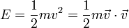
in which  corresponds to the mass of the particle, and
  is its velocity. Noting that classically the linear momentum
  is given by
  , so the kinetic energy can also be written as
 .
.
In order to get the quantum mechanical version of this, we substitute all occurrences of the momentum with
 ,
,
where  is the vector analogue of the partial differential operator
  .
.
Hence, the kinetic energy operator is given by
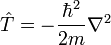 .
.
Total energy operator and the time dependent Schrödinger equation
The total energy operator introduces the time propagation to the wavefunctions so the
time dependent Schrödinger equation tells how the quantum system developes is time while
ist was found is some state at the original time.
It is basically constructed from the condition that its operation on time dependent
oscillatory factors characteristic to the plane waves obtained from the classical wave
equation describing the mechanical waves like sound or the waves on the water surface should produce the energy quanta
 as the eigenvalues from the eigen-equation
namely
as the eigenvalues from the eigen-equation
namely
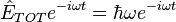
One therefore may readily guess it as
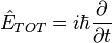
While te total energy in the classical mechanics is normally equal to the Hamiltonian the time dependent Schrödinger equation is obtained by equalizing the two:

How to solve the Schrödinger equation
Example 1: The ground state of the hydrogen atom
The time independent Schrödinger equation for the electron in the Coulomb potential in the spherical coordinates takes the form:
![-\frac{\hbar^2}{2 m} \left [
{1 \over r^2} {\partial \over \partial r}
\left(r^2 {\partial \over \partial r} \right)
+ {1 \over r^2 \sin \theta} {\partial \over \partial \theta}
\left(\sin \theta {\partial \over \partial \theta} \right)
+ {1 \over r^2 \sin^2 \theta} {\partial^2 \over \partial \varphi^2} \right ] \psi(r,\theta,\varphi) -\frac{e^2}{4 \pi \epsilon_0 r} \psi(r,\theta,\varphi)=
E \psi(r,\theta,\varphi).](../I/m/4422ce13ba76997666be5e4bd36013b7.png)
For the ground state which is the state with the lowest possible  we seek the
solution in the simplest possible form not dependent on the spherical angles
we seek the
solution in the simplest possible form not dependent on the spherical angles  and
and
 . The Schrödinger equation greatly simplifies to the second order ordinary partial differential equation of the one radial variable:
![-\frac{\hbar^2}{2 m} \left [
{1 \over r^2} {\partial \over \partial r}
\left(r^2 {\partial \over \partial r} \right)
\right ] \psi_0(r) -\frac{e^2}{4 \pi \epsilon_0 r} \psi_0(r)=
E_0 \psi_0(r).](../I/m/fa4e8d640b73e522b3eefc0f4acb4c81.png)
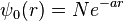
The part of it contains derivatives multiplied by the various powers of the  variable
and we guess the solution in the exponential form since the exponential function is the
eigenfunction of the differentiation operator while the derivative of the exponential
function is proportional to it:
variable
and we guess the solution in the exponential form since the exponential function is the
eigenfunction of the differentiation operator while the derivative of the exponential
function is proportional to it:
Substituting it to the Schrödinger equation we obtain the following equation:
![-\frac{\hbar^2}{2 m} \left [ -\frac{2 a}{r} + a^2\right ]\psi_0(r)-\frac{e^2}{4 \pi \epsilon_0 r} \psi_0(r)=E_0 \psi_0(r)](../I/m/31e36cba6529937b352be2c74ce167bb.png)
The only way this equation is valid for all values of is
that the coefficient multiplying the  is equal to
  :
:
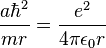
that gives the value of the Bohr radius  (the range how the ground state mostly extents radially):
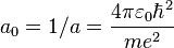
and the ground state energy
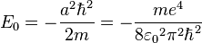 .
.
Example 2: Time dependent perturbation theory of weak field ionization
The first thing one can think to do above finding the ground state or the other allowed energies of the system is to solve the time dependent Schrödinger equation approximately i.e.
in the perturbative manner. Let us apply it to the small destruction effects on the
ground state of the quantum system and for the simplicity in one spatial dimension
which reduces the kinetic energy operator to the second derivative with the proper coefficients.
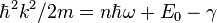
Let the ground state of the atom, for example the atom of Hydrogen will be
such that  is the smallest of possible values for the eigen-equation:

Let us add the external electric field effect to the Hamiltonian  in the simplest linear manner so the Schrödinger equation is
 .
.
We will assume
 for the initial condition
and will check what happens to that state under the influence of the perturbing
for the initial condition
and will check what happens to that state under the influence of the perturbing
 term, more specifically
where it will go in terms of the expansion in the basis of the unbound states of the system which
in very good approximation are simply plane waves.
For the convenience of the calculations we added the
term, more specifically
where it will go in terms of the expansion in the basis of the unbound states of the system which
in very good approximation are simply plane waves.
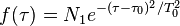
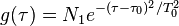
For the convenience of the calculations we added the  envelope function
normalized to
envelope function
normalized to  in time so the electric field is turned on and off in the smooth and
easy to Fourier transform Gaussian manner:
in time so the electric field is turned on and off in the smooth and
easy to Fourier transform Gaussian manner:
 .
.
it is now convenient to absorb the term in the equation in the so-called interaction picture introducing the transformed solution:
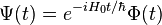
The original time-dependent equation greatly simplifies to
 .
.
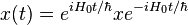
where the position operator becomes time dependent namely
With the zero iteration condition
 we get in the first approximation

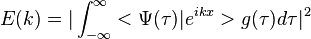
we are now interested in the unbound continuum state component in the final solution which tells us about the energy spectrum of the ionized electrons. We can get that by projecting the solution onto the continuum state, simply:

where we extended the integration in time from the minus infinity to infinity since the electric field was localized in time with the Gaussian envelope. The only significant term which remains after the integration is:
![E(k)=\frac{e^2 E_0^2}{4 \hbar^2}|<\Psi_0|x]e^{ik x}>{\tilde f}(\hbar^2 k^2/2m - \hbar \omega - E_0)|^2](../I/m/a080e1ca9b2c0e45dfc9e3c46b6043e5.png)
Where the  is the Fourier transform of the field envelope function
  and while is broadly localized the is sharply loalized around the point
with the condition
and while is broadly localized the is sharply loalized around the point
with the condition
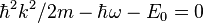
expressing the energy conservation condition

stating that while the ground state energy is negative there is no ionization below the threshold (for the photon or field frequencies that low that the kinetic energy would be impossibly negative) and the ejected electron kinetic energy is equal the energy of the absorbed photon lowered by the ionization or the binding energy.
Example 3: Theory of Above Threshold Ionization (ATI)
Above Threshold Ionization may be explained by solving the time dependent Schrödinger equation in the approximate manner. The Schrödinger equation for the free electron in the field of the electromagnetic wave in one dimension and in the radiation gauge is given by
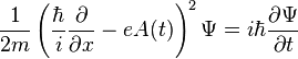 ,
,
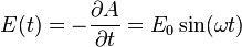
where
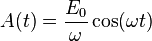
so the electric field is given by
Substituting
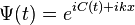
we are obtaining the equation for

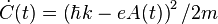
with the solution
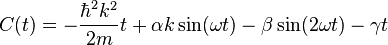 ,
,
where


 .
.
The Schrödinger equation for the electron in the wave field and in the atomic potential will be given by
![\left[H_0(t) + V(x) \right] \Psi= i\hbar{\frac{\partial \Psi}{\partial t}}](../I/m/c21df7cea41907624ede824862c2212d.png) ,
,
where,
is the Hamiltonian of the free electron in the field.
Adding and subtracting the energy of the ground state from which the
electron is to be ionized we obtain
![\left[H_0(t) + V(x) +E_0 - E_0 \right] \Psi= i\hbar{\frac{\partial \Psi}{\partial t}}](../I/m/9f59f53453453eb18c4ef8954dd3fc74.png)
Because in the ground state the electron kinetic energy is equall the total energy
but with the opposite sign (virial theorem)
and only this energy will be left after the fast removal of the electron, we neglect in this equation the sum
 for all
  and obtain the approximate equation
![\left[H_0(t) - E_0 \right] \Psi= i\hbar{\frac{\partial \Psi}{\partial t}}](../I/m/829a4f448bc0d0f83b579f1eac61a2c1.png) ,
,
where the only remaining of the atomic potential is the constant.
This equation may now be solved using the previous result for the free electron in the field and expanding the ground state into its Fourier components
 ,
,
with
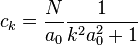
This equation has therefore the solution
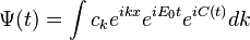
We obtain the ionization spectrum from the formula
 ,
,
telling how much of the plane wave of the free electron with the given kinetic energy is
at the and of the ionization process, where  is the averaging function of the measuring detector for example
 .
.
Expanding the factor
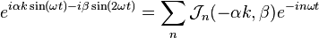
with the generalized Bessel functions  defined by the inverse transform, we obtain

( is the Fourier transform of the detector function) therefore the sum of sharp or fuzzy maxima
localized around the energy condition of emitted electrons
is the Fourier transform of the detector function) therefore the sum of sharp or fuzzy maxima
localized around the energy condition of emitted electrons
 depending on the speed i.e the averaging parameter of the detector
  .
.
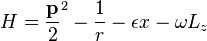
Example 4: Basic theory of the Trojan Wave Packet
Because the Trojan wave packet is an approximate eigenstate of the Hamiltonian its search starts from the Schrödinger´s equation for the Hydrogen atom in the field of the circularly polarized wave in the coordinate system rotating with the frequency of the field
-
 ,
,
where
-
 ,
,
and  is the operator of z-component of the angular momentum.
For the simplification one can restrict himself to only two spacial dimensions. This equation after neglecting the curvature terms of the Laplacian and assumption that some terms are slowly varying or even constant takes in the polar coordinate system the simplified and separated form
-
![\left[ -\frac {\partial^2}{2 \partial r^2} + \frac {l^2}{2 r^2} -\frac {1}{r} - {\epsilon} r -\frac {\partial^2}{2 r_0^2 \partial \phi^2}- {\epsilon} r_0 \cos \phi + \epsilon r_0 \right] \chi = E \chi](../I/m/7919d7a37ba4c21ae96e052fec2ce412.png) ,
,
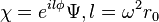
where  , and
, and  is the point of the potential of the
part of the Hamiltonian dependent only on the radial coordinate and therefore also the radius
of the classical orbit. Because the radial potential has the minimum the
Trojan wavepacket is in this theory the product of a well localized radial Gaussian function
and a well
localized excited state of the quantum mathematical pendulum, corresponding
to the pendulum totally reversed upside down which is also the Mathieu function with the characteristic value (and the energy)
equal with a good approximation to
is the point of the potential of the
part of the Hamiltonian dependent only on the radial coordinate and therefore also the radius
of the classical orbit. Because the radial potential has the minimum the
Trojan wavepacket is in this theory the product of a well localized radial Gaussian function
and a well
localized excited state of the quantum mathematical pendulum, corresponding
to the pendulum totally reversed upside down which is also the Mathieu function with the characteristic value (and the energy)
equal with a good approximation to  . The more precise theory shows that
it is the pendulum of a negative and fractional electron mass equal -1/3 (of the electron) and that is why it
is on the contrary the ground state with approximately the same energy but in the reversed spectrum.
. The more precise theory shows that
it is the pendulum of a negative and fractional electron mass equal -1/3 (of the electron) and that is why it
is on the contrary the ground state with approximately the same energy but in the reversed spectrum.
To notice that let us more keep the correction from the expansion of the centrifugal term
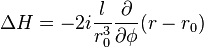
and let us consider its action on the Fourier component of  , e.g.
  .
.
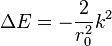
The additional centrifugal potential will be

It will cause the shift of the minimum and the energy lowering of the radial harmonic oscillator equal to
Replacing back  with the operator of the z component of the angular momentum we get
Adding this correction in the Schródinger equation we get the equation with the
negative and fractional electron mass -1/3 ( ):
):
-
![\left[ -\frac {\partial^2}{2 \partial r^2} + \frac {l^2}{2 r^2} -\frac {1}{r} - {\epsilon} r +\frac {3 \partial^2}{2 r_0^2 \partial \phi^2}- {\epsilon} r_0 \cos \phi + \epsilon r_0 \right] \chi = E \chi](../I/m/fe67d6e0ed73b46d542fa6b87c981c92.png) ,
,
which allows the Gaussian localization of the electron in the maximum but not in the minimum of the potential in the angular direction.
References
[1] Qi-Chang Su and J. H. Eberly, Numerical simulations of multiphoton ionization and above-threshold electron spectra, Phys. Rev. A 38, 3430 (1988)
[2] H. R. Reiss and V. P. Krainov, Approximation for a Coulomb-Volkov solution in strong fields, Phys. Rev. A 50, R910 (1994)