Rocks/Glaciers/Glaciology
< Rocks < Glaciers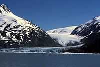
Glaciology studies the internal dynamics and effects of glaciers. More than one glacier with a common source is an ice field. Several ice fields can become an ice cap. When the ice cap becomes large enough it is an ice sheet.
Astronomy
"Sitting at an average height of around 4,000 metres above sea level, the plateau protrudes into the middle of the troposphere, where most weather events originate. As the biggest and highest plateau in the world, it disturbs this part of the atmosphere like no other structure on Earth."[1]
"The plateau’s remoteness, altitude and harsh conditions — it is often called the third pole because it hosts the world’s third-largest stock of ice — mean that even basic weather stations are few. Satellite data are also plagued by large errors owing to lack of calibration from ground observations."[1]
Radiation
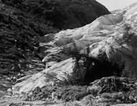
Def. "a glacier that experiences a dramatic increase in flow rate, 10 to 100 times faster than its normal rate; usually surge events last less than one year and occur periodically, between 15 and 100 years"[2] is called a surging glacier.
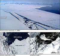
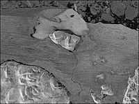
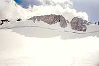
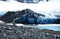
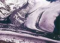
"In 1941, Hole-in-the-Wall Glacier [imaged at the right] surged, also knocking over trees during its advance."[2]
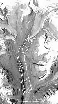
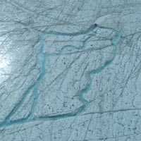
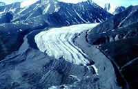
An "outlet glacier of the Sermersauq Ice Cap [on Disko Island, West Greenland, shown at the left with progressive surges marked] has surged 10.5 km downvalley to within 10 km of the fjord. [...] surging of the glacier, begun in 1995, was undetected until July 1999, when it was discovered during a geomorphic survey of the valley. Mapping from TM, Landsat and SPOT satellite imagery, and subsequent field work have documented the history of the event. On 17 June 1995 the terminus of the glacier was about where it appears in the 1985 air photography [...]. By 24 September 1995 the glacier had advanced 1.25 km and by 12 October another 1.25 km (mean advance during the second period : 70 m day-1). The advance slowed from 18 m day-1 in 1996 to 5 m day-1 in 1997 and <1 m day-1 between 1997 and 1999. By summer 1999 the advance ceased; the maximum extension of the terminus, about 10.5 km down-valley to about 10 km from the head of the fjord, was mapped from imagery on 9 July 1999 [...]."[3]
Planetary science
The ice ages or glaciations on Earth occurred from the early Proterozoic (Huronian), late proterozoic (Cryogenian), early Paleozoic (Andean-Saharan) during the Ordovician and Silurian periods, late Paleozoic (Karoo Ice Age) during the Carboniferous and early Permian periods, and lately the Quaternary glaciation.
Although these ice ages are widely separated in geological time, "in most parts of the Earth major climatic and palaeoenvironmental units typically have a duration of the order of half a precession cycle (around 10 ka) rather than half an eccentricity cycle (around 50 ka) so that the level of stratigraphic resolution provided by the Middle Pleistocene [Marine Isotope Stage] MIS (typical duration 50 ka) is not sufficiently fine to constitute a universal stratigraphic template."[4]
Colors
.jpg)
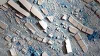
"Blue ice occurs when snow falls on a glacier, is compressed, and becomes part of a glacier ... blue ice was observed in Tasman Glacier, New Zealand in January 2011.[5] ... ice is blue for the same reason water is blue: it is a result of an overtone of an oxygen-hydrogen (O-H) bond stretch in water which absorbs light at the red end of the visible spectrum.[6]"[7]
Minerals
At the Dye 3 location in south east Greenland, "it takes roughly 100 years before the surface snow is compressed into solid ice. During this slow process (firnification) a given snow layer sinks to a depth of 80 m below the new surface formed under constant deposition of 1m of snow per year in South Greenland."[8]
In places, "surface melting often occurs in the summer time. The melt water seeps through the porous snow and refreezes somewhere in the cold firn, which disturbs the layer sequence, of course."[8]
"Firn air is the air that is trapped in the porous medium of firn, which is typically the first one hundred meters of an ice core."[9]
At the South Pole, the firn-ice transition depth is at 122 m, with a CO2 age of about 100 years.
Theoretical glaciology
Def. "a mass of ice that originates on land, usually having an area larger than one tenth of a square kilometer"[2] is called a glacier.
"[M]any believe that a glacier must show some type of movement; others believe that a glacier can show evidence of past or present movement."[2]
Def. the study of the internal dynamics and effects of glaciers is called glaciology.
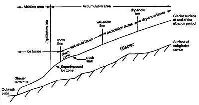
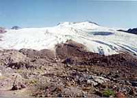
At the center above is an idealized diagram of an alpine or mountain glacier. "Glaciers are composed of an ablation and an accumulation area. Within these two areas several facies might be present [as indicated in the center diagram]. The facies represent distinctive areas with characteristics that reflect the environment under which the snow or ice was formed."[10]
"The accumulation area is typically composed of wet-snow facies, percolation facies and dry-snow facies [...] due to long periods of mild weather which influence the glacier surface at all altitude levels, the accumulation area [may consist] predominantly of wet- snow facies at the end of the ablation period."[10]
"Superimposed ice is formed by (1) the refreezing of meltwater during the autumn and/or during the ablation period and (2) the refreezing of meltwater on the glacier surface below the snow line at the end of the ablation period [...] net loss by melting occurs in the ice facies."[10]
Def. "a current of ice in an ice sheet or ice cap that flows faster than the surrounding ice"[2] is called an ice stream.
Def. "a network of interconnected glaciers or ice streams having a common source"[11] or "a large expanse of floating ice (several miles long)"[11] is called an ice field.
Def. "a dome-shaped mass of glacier ice that spreads out in all directions"[2] is called an ice cap.
Def. "a dome-shaped mass of glacier ice that covers surrounding terrain and is greater than 50,000 square kilometers (12 million acres)"[2] is called an ice sheet.
Aufeis
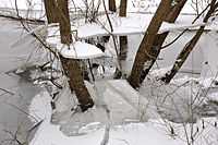
Def. a "sheet-like layered mass of ice"[12] is called aufeis.
Def. a "sheet-like layered mass of ice formed in freezing temperatures from the freezing of successive flows of ground water over previously formed layers of ice"[13] is called naled.
Little Ice Age
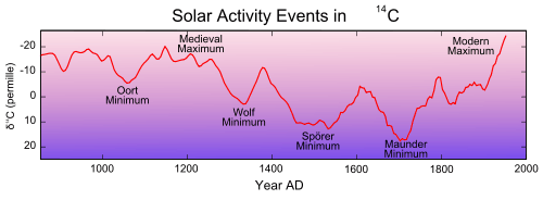
The Little Ice Age (LIA) appears to have lasted from about 1218 (782 b2k) to about 1878 (122 b2k).
A "climate interpretation was supported by very low δ’s in the 1690’es, a period described as extremely cold in the Icelandic annals. In 1695 Iceland was completely surrounded by sea ice, and according to other sources the sea ice reached half way to the Faeroe Islands."[8]
In the image at the top, "before present" is used in the context of radiocarbon dating, where the "present" has been fixed at 1950. The apparent decreases in solar activity are called the "Maunder Minimum", "Spörer Minimum", "Wolf Minimum", and "Oort Minimum".
"Northern Hemisphere summer temperatures over the past 8000 years have been paced by the slow decrease in summer insolation resulting from the precession of the equinoxes."[14]
Precisely "dated records of ice-cap growth from Arctic Canada and Iceland [show] that LIA summer cold and ice growth began abruptly between 1275 and 1300 AD, followed by a substantial intensification 1430-1455 AD. Intervals of sudden ice growth coincide with two of the most volcanically perturbed half centuries of the past millennium. [Explosive] volcanism produces abrupt summer cooling at these times, and that cold summers can be maintained by sea-ice/ocean feedbacks long after volcanic aerosols are removed. [The] onset of the LIA can be linked to an unusual 50-year-long episode with four large sulfur-rich explosive eruptions, each with global sulfate loading >60 Tg. The persistence of cold summers is best explained by consequent sea-ice/ocean feedbacks during a hemispheric summer insolation minimum; large changes in solar irradiance are not required."[14]
Quaternary
The "whole change elapsed just opposite the course of events that characterized the great glacial oscillations with sudden warming followed by slow cooling. Therefore, the two phenomena hardly have the same cause."[8]
"Most probably, the temperature drop 8250 years ago was caused by a release of enormous amounts of dammed meltwater from the retreating American ice sheet. In no time the light fresh water spread over large parts of the North Atlantic Ocean without being able to sink. Thereby the influx of warm water with the Gulf Stream stopped causing a sudden cooling of large oceanic and adjacent continental areas."[8]
Early history
The early history period dates from around 3,000 to 2,000 b2k.
Subatlantic history
The "calibration of radiocarbon dates at approximately 2500-2450 BP [2500-2450 b2k] is problematic due to a "plateau" (known as the "Hallstatt-plateau") in the calibration curve [...] A decrease in solar activity caused an increase in production of 14C, and thus a sharp rise in Δ 14C, beginning at approximately 850 cal (calendar years) BC [...] Between approximately 760 and 420 cal BC (corresponding to 2500-2425 BP [2500-2425 b2k]), the concentration of 14C returned to "normal" values."[15]
Subboreal history
The "period around 850-760 BC [2850-2760 b2k], characterised by a decrease in solar activity and a sharp increase of Δ 14C [...] the local vegetation succession, in relation to the changes in atmospheric radiocarbon content, shows additional evidence for solar forcing of climate change at the Subboreal - Subatlantic transition."[15]
The "Subboreal period is characterized by the highest accumulations of diatom frustules and chrysophyte cysts in Lake Baikal sediments. The siliceous microfossil record suggests that the Holocene climatic optimum in this interior part of Asia corresponds to the Subboreal period 2.5–4.5 ka and not to the Atlantic period 4.6–6 ka. Although quite different from Holocene reconstructions for the European part of Eurasia, the Holocene sedimentary record from Lake Baikal shows good correlation with palynological and soil climatic records from southeast Siberia and Mongolia where similar responses of the terrestrial biosphere are also documented. A distinctive monospecific lamina of Synedra acus diatom species, coincident with the maximum of chrysophyte cyst accumulation during the Subboreal period, argues for the possible short-term changes of the trophic state of Lake Baikal from oligotrophic, with a cold-water diatom assemblage, to eutrophic with a thermophilic monospecific diatom flora."[16]
Atlantic history
The "Atlantic period [is] 4.6–6 ka [4,600-6,000 b2k]."[16]
"During this [Atlantic] period the pollen indicates that the vegetation was quite clearly dominated by Alnus, with Betula and the trees of the mixed oak forest present in some quantity. The pollen of Corylus and Pinus, which were the dominants in the previous period, has decreased in amount. The low values for herbaceous types are maintained."[17]
"The end of the Atlantic period was marked by the decline of the elm, and was followed by a series of forest clearances which destroyed the mixed oak forest and produced the present vegetational landscape."[17]
"Some mountain glaciers in both the Northern and Southern Hemispheres advanced in late Atlantic and early sub-Boreal time, between about 5,200 and 4,600 radiocarbon years ago, and several in the Southern Hemisphere reached their greatest post-glacial extents."[18]
Boreal transition
"In some cores a narrow band of clay interrupts the organic muds, at the horizon of the Boreal Atlantic transition."[17]
"In the woodland the dominant trees are Betula, Pinus and Corylus. Ignoring the problem of over-representation of Pinus in the deep-water cores (cf. Pennington, 1947) the woodland remains a birch-pine woodland with an increasing amount of Corylus. Pinus decreases in the early part of zone V and Betula is also at lower values than previously. Towards the end of the period Pinus again becomes important."[17]
Ancient history
The ancient history period dates from around 8,000 to 3,000 b2k.
Pre-Boreal transition
The last glaciation appears to have a gradual decline ending about 12,000 b2k. This may have been the end of the Pre-Boreal transition.
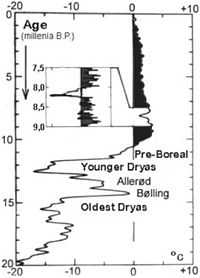
"About 9000 years ago the temperature in Greenland culminated at 4°C warmer than today. Since then it has become slowly cooler with only one dramatic change of climate. This happened 8250 years ago as shown in detail to the left of the main record in [the figure at the right]. In an otherwise warm period the temperature fell 7°C within a decade, and it took 300 years to re-establish the warm climate. This event has also been demonstrated in European wooden ring series and in European bogs."[8]
"The last remains of the American ice sheet disappeared about 6000 years ago, the Scandinavian one 2000 years earlier."[8]
"The Pre-boreal period marks the transition from the cold climate of the Late-glacial to the warmer climate of Post-glacial time. This change is immediately obvious in the field from the nature of the sediments, changing as they do from clays to organic lake muds, showing that at this time a more or less continuous vegetation cover was developing."[17]
"At the beginning of the Pre-boreal the pollen curves of the herbaceous species have high values, and most of the genera associated with the Late-glacial fiora are still present e.g. Artemisia, Polemomium and Thalictrum. These plants become less abundant throughout the Pre-boreal, and before the beginning of the Boreal their curves have reached low values."[17]
Younger Dryas
"The Younger Dryas interval during the Last Glacial Termination was an abrupt return to glacial-like conditions punctuating the transition to a warmer, interglacial climate."[19]
"From former cirque glaciers in western Norway, it is calculated that the summer (1.May to 30.September) temperature dropped 5-6°C during less than two centuries, probably within decades, at the Alleröd/Younger Dryas transition, some 11,000 years ago."[20]
"From the same data the Younger Dryas summer temperature is estimated to have been 8-10°C lower than at present, and from fossil ice wedges the mean annual temperatures 13°C lower than at present in the same area."[20]
"At the time of the Alleröd/Younger Dryas transition, the Scandinavian ice-sheet was still a major element in the climate system. The record from the Younger Dryas is distinct, consisting of ice-marginal deposits that are mapped nearly continuously around Scandinavia [...], showing that the climate turned to a more glacial regime in both the continental climate area of USSR/Finland and the oceanic climate area of Western Norway. This suggests that lower summer temperatures, and not increased winter precipitation, was the climatic factor that determined the major pattern of glacial response."[20]
An "amplification of the re-advance in Western Norway compared to the easterly areas, due to higher winter precipitation along the western flank of the ice-sheet, and topographical and glaciological factors [...] The re-advance also caused a relative rise in sea level in Western Norway through the combination of increased gravitational attraction and a halt in glacio-isostatic uplift (Anundsen, 1985)."[20]
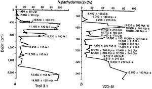
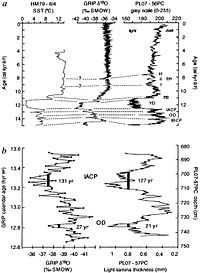
The diagrams on the right show percentages of the planktonic foraminifera Neogloboquadrina pachyderma from two cores: "a" Troll 3.1 (60° 46.7' N, 3° 42.8' E, 332 m water depth) in the Norwegian Trench and "b" V23-81 located off Ireland.[21]
"Annual layer counting through the most recent of these [sudden changes in the temperature of precipitation] indicates that a warming of ~7 °C occurred within a 50-yr period during the transition from the Younger Dryas cold phase (~11-10 kyr BP) to the present interglacial2."[21]
Allerød Oscillation
"During the Allerød Chronozone, 11,800 to 11,000 years ago, western Europe approached the present day environmental and climatic situation, after having suffered the last glacial maximum some 20,000 to 18,000 years ago. However, the climatic deterioration 11,000 years ago led to nearly fully glacial conditions on this continent for some few hundreds of years during the Younger Dryas. This change is completely out of phase with the Milankovitch (orbital) forcing as this is understood today, and therefore its cause is of major interest."[20]
"During the Allerød a branch of the North Atlantic Current entered the Norwegian Sea (Ruddiman and Mclntyre, 1973, 1981)."[20]
"Recent stratigraphical achievements and long time established chronologies exist for the Late Weichselian, i.e. 10-25 ka BP. During this period Denmark experienced the complex Main-Weichselian glaciation from 25 to about 14 ka BP (Jylland stade, Houmark-Nielsen 1989) followed by the Late Glacial climatic amelioration including the interstadial Bølling-Allerød oscillation (13-11 ka BP), finally leading to the interglacial conditions that characterize the Holocene (Hansen 1965)."[22]
The "large, but so far largely ignored eruption of the Laacher See-volcano, located in present-day western Germany and dated to 12,920 BP, had a dramatic impact on forager demography all along the northern periphery of Late Glacial settlement and precipitated archaeologically visible cultural change. In Southern Scandinavia, these changes took the form of technological simplification, the loss of bow-and-arrow technology, and coincident with these changes, the emergence of the regionally distinct Bromme culture. Groups in north-eastern Europe appear to have responded to the eruption in similar ways, but on the British Isles and in the Thuringian Basin populations contracted or relocated, leaving these areas largely depopulated already before the onset of the Younger Dryas/GS-1 cooling."[23]
Evidence "from the Hudson Valley and the northeastern U.S. continental margin [...] establishes the timing of the catastrophic draining of Glacial Lake Iroquois, which breached the moraine dam at the Narrows in New York City, eroded glacial lake sediments in the Hudson Valley, and deposited large sediment lobes on the New York and New Jersey continental shelf ca. 13,350 yr B.P. Excess 14C in Cariaco Basin sediments indicates a slowing in thermohaline circulation and heat transport to the North Atlantic at that time, and both marine and terrestrial paleoclimate proxy records around the North Atlantic show a short-lived (<400 yr) cold event (Intra-Allerød cold period) that began ca. 13,350 yr B.P."[24]
Neolithic
The base of the Neolithic is approximated to 12,200 b2k.
Mesolithic
The mesolithic period dates from around 13,000 to 8,500 b2k.
Older Dryas
The Older Dryas is a "century-scale cold [event]".[25]
"The most negative δ 18O excursions seen in the GRIP record lasted approximately 131 and 21 years for the [inter-Allerød cold period] IACP and [Older Dryas] OD, respectively. The comparable events in the Cariaco basin were of similar duration, 127 and 21 years. In addition to the chronological agreement, there is also considerable similarity in the decade-scale patterns of variability in both records. Given the geographical distance separating central Greenland from the southern Caribbean Sea, the close match of the pattern and duration of decadal events between the two records is striking."[26]
In the figures on the right, especially b, is a detailed "comparison of δ 18O from the GRIP ice core24 with changes in a continuous sequence of light-lamina thickness measurements from core PL07-57PC. Both records are constrained by annual chronologies, although neither record is sampled at annual resolution. The interval of comparison includes the inter-Allerød cold period (12.9-13 cal. kyr BP) and Older Dryas (13.4 cal. kyr BP) events (IABP and OD from a). The durations of the two events, measured independently in both records, are very similar, as is the detailed pattern of variability at the decadal timescale."[26]
Bølling Oscillation
The "intra-Bølling cold period [IBCP is a century-scale cold event and the] Bølling warming [occurs] at 14600 cal [calendar years] BP (12700 14C BP)".[25]
The "Bølling was originally defined as starting from 13000 14C BP (calibrated to ~15650 cal BP; Stuiver et al., 1998). [...] independent annual chronology indicate a much later onset of the Bølling (e.g., 14600 cal BP".[25]
"During the IBCP and perhaps also IACP, δ 18O values inversely correlate with δ 13C, but during the OD δ 18O shows positive correlation with δ 13C, suggesting dry conditions with high evaporation, as well as cold."[25]
The "δ 18O record shows late-glacial climatic deterioration beginning in latest Bølling time and culminating in a Younger Dryas reversal. The vegetation record shows only a small increase in non-arboreal pollen in Younger Dryas time, reflecting some openings in the forest cover. The alpine moraine record shows widespread Egesen moraines of Younger Dryas age (Ivy-Ochs et al. 1999). In sharp contrast to the situation in Great Britain, Younger Dryas cooling is not reflected in the insect record at Lobsigensee."[27]
"During the early Bølling warming, the boreal insect assemblage is replaced by a plant-independent temperate assemblage that reflects a mean July temperature close to interglacial values, just as in Great Britain. A shift in water plants supports such marked warming. The early Bølling climate was warm enough to support broad-leafed deciduous trees such as oak or hazel, which do not appear until 3000 years later because of migrational lags."[27]
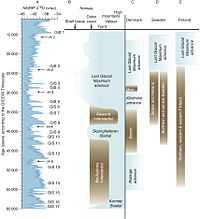
The Bølling interstadial corresponds to GIS 1 as shown in the diagram on the right.[28]
Oldest Dryas
"During the Late Weichselian glacial maximum (20-15 ka BP) the overriding of ice streams eventually lead to strong glaciotectonic displacement of Late Pleistocene and pre-Quaternary deposits and to deposition of till."[22]
"The synchronous and nearly uniform lowering of snowlines in Southern Hemisphere middle-latitude mountains compared with Northern Hemisphere values suggests global cooling of about the same magnitude in both hemispheres at the [Last Glacial Maximum] LGM. When compared with paleoclimate records from the North Atlantic region, the middle-latitude Southern Hemisphere terrestrial data imply interhemispheric symmetry of the structure and timing of the last glacial/interglacial transition. In both regions atmospheric warming pulses are implicated near the beginning of Oldest Dryas time (~14,600 14C yr BP) and near the Oldest Dryas/Bølling transition (~12,700-13,000 14C yr BP). The second of these warming pulses was coincident with resumption of North Atlantic thermohaline circulation similar to that of the modern mode, with strong formation of Lower North Atlantic Deep Water in the Nordic Seas. In both regions, the maximum Bølling-age warmth was achieved at 12,200-12,500 14C yr BP, and was followed by a reversal in climate trend. In the North Atlantic region, and possibly in middle latitudes of the Southern Hemisphere, this reversal culminated in a Younger-Dryas-age cold pulse."[27]
"The Oldest Dryas part of the Lobsigensee records [on the Swiss Plateau] features a boreal and boreal-montane insect assemblage, along with Betula nana."[27]
Jylland stade
"After c. 22 ka BP during the Jylland stade (Houmark-Nielsen 1989), Late Weichselian glaciers of the Main Weichselain advance overrode Southeast Denmark from the northeast and later the Young Baltic ice invaded from southeasterly directions. Traces of the Northeast-ice are apparently absent in the Klintholm sections, although large scale glaciotectonic structures and till deposits from this advance are found in Hjelm Bugt and Møns Klint (Aber 1979; Berthelsen 1981, 1986). At Klintholm, the younger phase of glaciotectonic deformation from the southeast and south and deposition of the discordant till (unit 9) were most probably associated with recessional phases of the Young Baltic glaciation. In several cliff sections, well preserved Late Glacial (c. 14-10 ka BP) lacustrine sequences are present (Kolstrup 1982, Heiberg 1991)."[22]
The "Allarp Till (Berglund & Lagerlund 1981), was deposited in connection with the first Late Weichselian ice advance in southern Sweden. Petrographic studies (Bose 1990) indicate that the first Late Weichselian ice advance which overrode northern Germany and reached the Brandenburg stage has a composition comparable to the Allarp till and the bedded diamictons from Klintholm."[22]
GIS 2
The weak interstadial corresponding to GIS 2 occurred about 23.2 kyr B.P.[28]
GIS 3
The stronger GIS 3 interstadial occurred about 27.6 kyr B.P.[28]
Møn interstadial
The Møn interstadial corresponds to GIS 4.[28]
Klintholm advance
This advance occurred after the Møn and ended with GIS 6.[28]
GIS 5
GIS 5 interstadial occurred during the Klintholm advance about 33.5 kyr B.P.[28]
Ålesund Interstadial
The Ålesund interstadial began with GIS 6 and ended after GIS 8.[28]
Huneborg interstadial
The Huneborg interstadial is a Greenland interstadial dating 36.5-38.5 kyr B.P. GIS 8.[28]
Hengelo interstadial
The Hengelo interstadial [is] > 35 ka BP".[22]
"An evolution with the coldest phases (coarsest grains) between 27,000 and 10,000 years B.P., 52,000 and 34,000 years B.P., and 76,000 and 60,000 years B.P. and relatively warmer intervals (finer grain size) in between is obvious. Apparently, they reflect a 21,000-year periodicity. This trend is superposed by much shorter oscillations of a duration of one to a few thousand years. Their duration is similar to the Dansgaard-Oeschger oscillations in the ice-core records. Some well-defined stadials and interstadials from the terrestrial records show also such a duration: for instance, the Hengelo interstadial around 37-38,500 14C years B.P. (Zagwijn, 1974; Kasse et al., 1995) and the preceding Hasselo stadial at approximately 40-38,500 14C years B.P. (Van Huissteden, 1990)."[29]
Hasselo stadial
The "Hasselo stadial [is] at approximately 40-38,500 14C years B.P. (Van Huissteden, 1990)."[29]
The most pronounced cold interval in The Netherlands is the Hasselo Stadial (van Huissteden, 1990) at ca. 41-38.5 ka, followed by the warm Hengelo Interstadial (Zagwijn, 1974)."[30]
"One of two strongly rounded fragments of the mammoth maxilla from the Shapka Quarry in the southern Leningrad region was recently dated at 38450 + 400/–300 years (GrA-39 116) and rhinoceros remains (spoke bone), back to 38360 + 300/–270 years ago (GrA-38 819) [7]. The maxilla fragments occurred in sediments of the Leningrad Interstadial, which correspond to the transition between the Hasselo Stadial (44–39 ka ago) and the Hengelo Interstadial (38–36 ka ago)."[31]
The Hasselo stadial corresponds to the Skjonghelleren stadial in Norway but to the Sejrø interstadial in Denmark.[28]
Moershoofd interstadial
The Moershoofd interstadial has a 14C date of 44-46 kyr B.P. and corresponds to GIS 12 at 45-47 kyr B.P.[28]
"Ice retreat along the Norwegian coast (Bø/Austnes, Ålesund [interstadials]) coincided with a series of especially warm Greenland Interstadials (Mangerud et al. 2003, 2009; Mangerud 2004) [GIS 12-14]. However, the advance and retreat phases of the [Scandinavian Ice Sheet] SIS along the Norwegian coast and in southernmost Scandinavia seem to have been partly asynchronous [...]. The Ristinge advance into Denmark is, for example, dated to the same time interval as the Bø/Austnes interstadial in Norway."[28]
Glinde interstadial
The Glinde interstadial has a 14C date of 48-50 kyr B.P. and corresponds to GIS ?13/14 with a GIS age of 49-54.5 kyr B.P.[28]
Oerel interstadial
The Oerel interstadial has a 14C date of 53-58 kyr B.P. and corresponds to GIS 15/16 with a GIS age of 56-59 kyr B.P.[28]
Karmøy stadial
The Karmøy stadial begins in the high mountains of Norway about 58 kyr B.P. and expands to the outer coast by 60 kyr B.P.[28]
Odderade interstadial
The Odderade interstadial has a 14C date of 61-72 kyr B.P. and corresponds to GIS 21.[28]
Brørup interstadial
The "Brørup interstade [is about] 100 ka BP".[22] It corresponds to GIS 23/24.[28]
Eemian interglacial
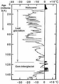

"Note the controversially split Eemian period [in the figure at the right], the predecessor of our own warm period about 125,000 years ago. Did the Eem climate in Greenland really oscillate between 5° warmer and 5° colder than now? In Europe the climatic variability was less than in Greenland, during the glaciation as well as in the Eemian period."[8]
"The Eem interglaciation is usually described as a warm and climatically stable period. It lasted from 131 to 117 kyr B.P. on our time scale. The sea level was 6-8 m higher than today, and a subtropical fauna invaded parts of Europe."[8]
Was "the Eemian climate as unstable as suggested in [the figure at the right]? Or is the tripartition in the δ-record an artifact caused by the deep layers being disturbed by ice movements, for example by folding?"[8]
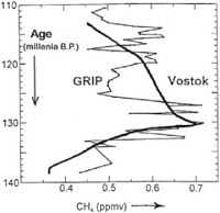
The second image at the right shows "atmospheric concentration of methane during the Eem period measured on the ice cores from Vostok, East Antarctica (heavy curve) and GRIP, Central Greenland (the thin, strongly varying curve). The two curves “ought to have” the same trends, because the atmosphere is well mixed any time."[8]
The "methane content in Emian ice in the Antarctic Vostok core changes quite smoothly, whereas it changes in phase with the tripartite δ-record at Summit. Since the atmosphere is quite well mixed at any time, its methane content cannot have varied so differently at the two poles. Thus the high δ Eemian ice at Summit must have been exposed to a couple of inserts of low δ ice from a cold period with low methane content in the atmosphere".[8]
"Ocean sediment cores from [the Norwegian Sea] exhibit a split Emian almost like δ in the Summit ice core [as compared in the first figure at the left]."[8]
"On the left [in the first figure at the left]: An ocean sediment core from the western part of the Norwegian Sea outlines the Eem as an unstable period, cf. the per cent occurrence of a foraminifera species (N pachyderma (s)) that thrives best in cold water. Note the reversed scale at the bottom (after Fronval et al.,1999) On the right: Greenland temperature deviations from present values calculated from the GRIP ice core δ record. Both of the time scales are given in millennia before present."[8]
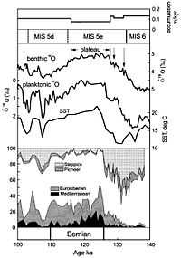
"Core MD95-2042 was collected using the CALYPSO Kullenberg corer aboard Marion Dufresne MD in 1995] at 37°48'N, 10°10'W in a water depth of 3146 m (Bassinot et al., 1996)."[4]
The second figure on the left shows marine "and continental records of the last interglacial in core MD95-2042 on a time scale based on radiometric dates for uplifted corals [...]. From the top: Sedimentation rate [is] implied by the age controls marked; benthic δ 18O record (replicates averaged); planktonic δ 18O record (replicates averaged); sea surface temperature [SST] based on U37k alkenones; major groups of pollen taxa."[4]
"The beginning of the Eemian is identified in the vegetational sequence by a simultaneous drop in steppic elements and a rise in Eurosiberian and Mediterranean trees; there is no ambiguity in its placement. This change coincides with a 5° rise in sea-surface temperature as indicated by the alkenone measurements; the coincidence with the planktonic δ 18O change (also indicating a sea-surface temperature rise) is equally striking. The age of this event on our timescale is 126 ka, significantly later than the attainment of the [Marine Isotope Stage] MIS 5e plateau in benthic δ 18O. This implies that in contrast to the base of the Holocene, the major ice sheets had completely melted before the beginning of interglacial climatic conditions in Northwest Europe. In view of the fact that immediately prior to this transition, cold water was offshore at the latitude of southern Portugal, it is very unlikely that the beginning of the vegetation-defined interglacial was any earlier at sites further to the North."[4]
"The end of the Eemian is identified in the vegetational sequence by a simultaneous rise in steppic elements and a drop in Eurosiberian trees, and the disappearance of the Mediterranean elements. Again the placement of the boundary is relatively uncontroversial at least at a local level. This boundary is well within MIS 5d and indeed appears shortly before the most positive benthic δ 18O values are recorded, implying that the Laurentide ice sheet had grown considerably."[4]
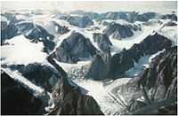
Holarctic-Antarctic Ice Age
"This late Cenozoic ice age began at least 30 million years ago in Antarctica; it expanded to Arctic regions of southern Alaska, Greenland, Iceland, and Svalbard between 10 and 3 million years ago. Glaciers and ice sheets in these areas have been relatively stable, more-or-less permanent features during the past few million years."[32]
"During the last one million years, large ice sheets developed in North America, Eurasia, the Andes, and elsewhere. These ice masses were unstable, growing and self-destructing in cycles averaging about 100,000 years, which correspond to eccentricity in the Earth's orbit around the Sun (Mangerud et al. 1996). The most recent great ice sheets disappeared only 10,000 years ago, but the Holarctic-Antarctic Ice Age still continues in regions of stable glaciation."[32]
Karoo Ice Age
A "glacial marine facies [occurs] on the Falkland Islands [Frakes and Crowell, 1967]."[33]
In "a complex situation, like the Karoo Basin and adjoining highlands [...] a marine ice sheet bounded the highlands during the last phase of glaciation".[33]
The "influence of Gondwana topography on glaciation about 275 to 300 m.y. ago, [...] is preserved as thick (up to 700 m) glacial and proglacial sequences in the Karoo, Kalahari, and Warmbad basins as well as other smaller basins toward the north. These deposits, known as the Dwyka Formation, cover an area close to a million square kilometers in southern Africa".[33]
"Valleys that had been incised into the Windhoek Highlands attained lengths up to 250 km, had striated floors and walls, and contained roches moutonnées [Martin, 1961]."[33]
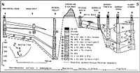
"The Whitehill Formation (White Band) was taken as a datum [in the stratigraphic diagram on the lower right]. The Permo-Carboniferous boundary on the platform is based on microflora assemblages [Anderson, 1977]. Ms is massive; St, stratified; dmt, diamictite; Drg, dropstone argillite; Cb, carbonaceous; mds, mudstone; Sst, sandstone; Lm, laminated; cgl, conglomerate; sh, shale; Fs, fossiliferous; Cc, carbonate; and conc, concretions."[33]
"Glaciation is known from all continents that were once part of Gondwana, including: Africa, South America, Antarctica, India, Arabia and Australia. Glaciation began in the early Carboniferous (360 Ma), reached a peak in late Carboniferous, continued into early Permian, and mostly came to an end by late Permian (260 Ma) time, thus spanning 100 million years. Multiple glacial centers were active; each experienced repeated glacier advances and retreats. Particularly well-known glacial strata include the Dwyka Tillite (Karoo basin) in South Africa, Talchir Boulder Beds in India, and Wynyard Formation of Tasmania. Overall, two major glacial cycles took place. Both expanded gradually over periods of about 20 million years each to reach their maximum extents in late Pennsylvanian and early Permian times. Each major cycle then ended abruptly during only 1-10 thousand years (Gastaldo et al. 1996)."[32]
"Although precise dating is not possible for many of the Gondwana glacial deposits, a general migration of glaciation through time is apparent. Carboniferous glaciation took place mainly in South America, southern Africa, India, and western Antarctica; whereas Permian glaciation was located mostly in Australia and eastern Antarctica. This migration corresponded to the drifting of Gondwana over the South Pole [...] The Karoo ice age is marked by cyclothems, cyclic sedimentary sequences in continental areas that were located in low latitudes. Pennsylvanian and Permian cyclothems are well known throughout the mid-continent of the United States, particularly eastern Kansas. The cyclothems were created by repeated marine transgressions and regressions over a stable continental platform. These cycles are interpreted as results of frequent changes in global sea level associated with glaciation in Gondwana. Glacial cycles and variations in sea level are documented in oxygen-isotope variations within fossils of Pennsylvanian cyclothems [...]. Late Pennsylvanian sea-level fluctuations were at least 80 m and likely greater than 100 m in amplitude (Soreghan and Giles 1999)."[32]
Andean-Saharan ice age
The "glacial episodes that occurred on Earth during the Palaeozoic (the Andean-Saharan between 450 and 420 Ma, and the Karoo between 360 and 260 Ma) did not achieve a global extent."[34]
"Glaciation is known from Arabia, central Sahara, western Africa, the lower Amazon of Brazil, and the Andes of western South America. Spectacular erosion of underlying rocks took place over large areas of the Sahara; whereas a good sedimentary record is preserved in Arabia. Continental ice sheets were developed in Africa and eastern Brazil, while alpine glaciers formed in the Andes region. The center of glaciation appears to have migrated through time: Ordovician (450-440 Ma) in Sahara, and Silurian in South America (Brazil 440-430 Ma, and Andes 430-420 Ma). The two continents were joined as parts of Gondwana, which was located over the South Pole".[32]
Cryogenian ice age
The Cryogenian Ice Age, or the Stuartian-Varangian Ice Age, a "Late Proterozoic ice age was apparently the greatest of all. Glacial strata are known from all modern continents (except Antarctica) with an overall time range of about 950 to 600 million years old. Glacial strata from several intervals during this time are well preserved in Africa, China, Australia, Europe, Arabia, North America, and elsewhere. Multiple glaciations are the rule. In Scotland and Ireland, for example, three glacial episodes took place between 700 and 580 million years ago (McCay et al. 2006)."[32]
It apparently consists of
- glaciation of the Lower Congo region, Africa occurring 950-750 and 620-600 Ma,
- Stuartian glaciation, Australia, 800-780 Ma,
- Sinian glaciation, China, 800-760, 740-700, and 600 Ma,
- glaciation in Western Canada/U.S.A., 850-800 Ma,
- glaciation of the Saharan region, Africa, 730-650 Ma,
- Marinoan glaciation, Australia, 690-680 Ma, and
- Varangian glaciation, Norway, about 650 Ma.[32]
Huronian ice age
The Huronian Ice Age is known "mainly from Canada and the United States in North America, where dated rocks range from 2500 to 2100 million years old. The Gowgonda Formation of Ontario is especially noteworthy for its excellent preservation of glaciogenic strata dated about 2300 million years old. Other glacial deposits are found in Wyoming, Michigan, Quebec, and the Northwest Territories. These rocks record extensive Early Proterozoic continental glaciation through a time span of about 400 million years, during which three or more glacial expansions took place. The configuration of the continents during this time is highly speculative."[32]
Glacial ice petrogony
Usually glacial ice starts with the meteoritic accumulation of snow. Depending on temperature, latitude, altitude, and occasional other factors, snow melts to water, sublimates to water vapor, or accumulates progressively.
"Snow develops into ice much more rapidly on glaciers in temperate regions, where periods of melting alternate with periods when wet snow refreezes, than in [regions] where the temperature remains well below the freezing point throughout the year."[35]
Different "mechanisms [occur] in different areas. We have to subdivide glaciers, and even different parts of the same glacier, into different categories according to the amount of melting that takes place."[35]
"The zones differ one from another in the temperature and physical characteristics of the material near the surface."[35]
"New snow (immediately after falling in calm conditions) [has a typical density of] 50-70 [kg m-3.] Damp new snow [ranges from] 100-200 [s]ettled snow 200-300 [d]epth hoar 100-300 [w]ind-packed snow 350-400 [f]irn 400-830 [v]ery wet snow and firn 700-800 [and] [g]lacier ice 830-923 [...] The difference between firn and ice is clear; firn becomes glacier ice when the interconnecting air- or water-filled passageways between the grains are sealed off, a process known as pore close-off."[35]
"Crystal size [grain size] increases with time and depth as snow transforms to ice."[35]
"The characteristics of the [glacier] zones [start] from the highest elevations (the head of a glacier or center of an ice sheet)."[35]
- Dry-snow zone: "No melting occurs here, even in summer. The dry-snow line marks the boundary between this zone and the next one."[35]
- Percolation zone: "Some surface melting occurs in this zone. Water can percolate a certain distance into snow at temperatures below 0 °C before refreezing. If the water encounters an impermeable layer it may spread out laterally. When it refreezes an ice layer or an ice lens forms. The vertical water channels also refreeze, when their water supply is cut off, to form pipe-like structures called ice glands."[35]
- Wet-snow zone: In this zone, by the end of summer, all the snow deposited since the end of the previous summer has warmed to 0 °C."[35]
- Superimposed-ice zone: In the percolation and wet-snow zones, the material consists of ice layers, lenses, and glands, separated by layers and patches of snow and firn. At lower elevations, [...] so much meltwater is produced that the ice layers merge to a continuous mass, called superimposed ice. [...] The snow line refers to the boundary between the wet-snow and the superimposed-ice zones."[35]
- Ablation zone: the area below the equilibrium line [the lower boundary of the superimposed-ice zone.] Here the glacier surface loses mass by the end of the year."[35]
Def. "the section of the glacier where melting dominates"[36] is called the ablation zone.
"By the end of the summer this area [ablation zone] is exposed glacier ice."[36]
Def. "the zone of the glacier where snowfall exceeds snowmelt"[36] is called the accumulation zone.
Greenland ice sheet petrogony
Def. the study of the origin of rocky objects, or rocks, is called petrogony.
"The ice cap covers 85% of the total 2.2 mill. km2 area of Greenland [...]. It measures 2500 km from north to south and about 750 km from west to east in Mid Greenland. The surface reaches 3250 m [above sea level] a.s.l. at Summit and 2850 m on a minor dome in South Greenland."[8]
"Unlike the American and Scandinavian ice sheets built up during each glaciation in the past, most of the Greenland ice cap survived the intervening warm periods for two reasons: Firstly, the high surface elevation (at present 2/3 of its area lies more than 2000m a.s.l.) is associated with low surface temperatures (present annual mean values down to -32°C at Summit), and melting with run-off only in the marginal areas. Secondly, ample supply of precipitation from the Atlantic Ocean is given off by low-pressures moving northward along the coasts, sometimes even crossing the ice sheet."[8]
"The annual accumulation ranges from 13 cm of water equivalent in the central part of northeast Greenland to more than 100 cm along the southeastern coast, a total supply of about 500 km3 of water equivalent per year. The total annual loss of material is approximately of the same magnitude, of which 50% is given off as melt water by mainly coastal surface and bottom melting and an equal amount as icebergs."[8]
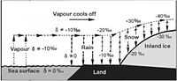
The diagram at the right shows "δ-changes (isotopic fractionation [...]) in vapour and precipitation by evaporation from the sea (to the left) and by formation of precipitation [snow] from a cooling air mass during its move towards higher latitudes and/or higher altitudes, e.g. along a warm front or over the inland ice (to the right)."[8]
"The main reason why δ varies in the water cycle is that the heavy H2O18 molecules have a 10 ‰ lower tendency to evaporate from a water surface than the light H2O16 molecules, and a 10 ‰ higher tendency to condensate from water vapour – or in physical terms: The vapour pressure of H2O18 is 10 ‰ lower than that of H2O16. Hence, vapour in equilibrium with sea water (SMOW) has a δ-value of -10 ‰. [indicated in the diagram to the right] and, conversely, when the vapour cools off droplets are formed with a δ-value 10 ‰ higher than that of the vapour, at first therefore 0 ‰."[8]
"When a cloud gives off rain, it loses more H2O18 than corresponding to the concentration in the vapour. The remaining vapour thereby gets a lower δ-value. This decrease in δ will continue by further cooling, and so will the δ of the rain as the precipitation process proceeds. If the air mass does not take up new vapour on the way, the δ-value of the precipitation decreases approximately by 0.7 ‰ per °C cooling."[8]
"In [the diagram at the right] the primary evaporation takes place from a sub-tropical ocean surface to the left, and the horizontal arrows follow the humid air mass toward north while cooling to the dew point, when the first rain is formed (with δ = 0 ‰). During the proceeding cooling, when the air mass crosses a continent, or flows over the inland ice (to the right in the figure), or ascent along a warm front, it gives off precipitation and acquires steadily decreasing δ’s for both the vapour and the precipitation. This explains [...] the generally very low δ values in rain from the top part of the warm front [...]."[8]
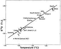
The second figure at the right "shows how the mean δ of snow is correlated with the local mean annual air temperature measured 10 or 20m below surface. Disregarding some stations on the eastern slope of the ice cap indicated by crosses, 1 centigrade lower temperature corresponds to 0.7 ‰ lower δ-value. The deviation of the stations on the eastern slope is probably due to these stations receiving some snow from western directions, i.e. from air-masses that have passed the high ice-ridge thereby losing considerable amounts of the isotopically heavy components of the water vapour, whereas the temperature is determined by adiabatic ascent from the east."[8]
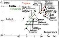
"In [the third lower figure at the right] the Atlantic [United Nations’ International Atomic Energy Agency] IAEA stations are divided into groups of ocean, coast and continental stations. Further grouping in a tropical-subtropical (red), a temperate (green) and a polar (violet) category shows linear relationships between annual δ versus temperature within each category, which suggests (1) the influence of re-evaporated fresh water from the continents, and (2) the existence of at least two more or less separate distillation columns in the Atlantic Ocean, a tropical-subtropical and a temperate one, perhaps even a polar one. This is an effect of the air taking up new vapour during its travel toward higher latitudes, i.e. a precipitation pattern more complicated than that considered in [the first diagram at the right]."[8]
Objects
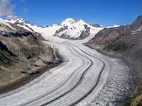
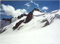
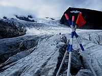
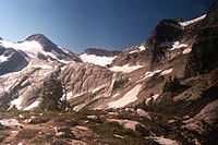
The Aletsch glacier in the image on the right is the largest in the Swiss Alps.
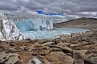
The Quelccaya ice cap in the image on the left is located in southern Peru in the Cordillera Vilcanota and is the largest glaciated area in the tropics.
Continuum
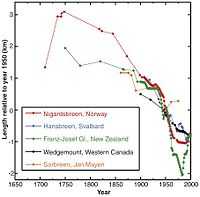
There is a "link between climate processes and glacier mass balance (3, 4)."[37]
"The response of a glacier to climate change depends on its geometry and on the climatic setting. To unravel the climate signal con- tained in the glacier length records, it is necessary to discriminate with respect to the climate sensitivity c and to the response time τ (the time a glacier needs to approach a new equilibrium state). Similar to other climate proxies, glacier length fluctuations are the product of variations in more than one meteorological parameter. Glacier mass balance depends mainly on air temperature, solar radi- ation, and precipitation."[37]
The "primary source for melt energy is solar radiation but that fluctuations in the mass balance through the years are mainly due to temperature and precipitation (25, 26). Mass-balance modeling for a large number of glaciers has shown that a 25% increase in annual precipitation is typically needed to compensate for the mass loss due to a uniform 1 K warming (3, 27). These results, combined with evidence that precipitation anomalies normally have smaller spatial and temporal scales than those of temperature anomalies (2), indicate that glacier fluctuations over decades to centuries on a continental scale are primarily driven by temperature. Here, the climate sensitivity c is therefore defined as the decrease in equilibrium glacier length per degree temperature increase."[37]
"Climate sensitivity depends in particular on the surface slope (a geometric effect) and the annual precipitation (a mass-balance effect)."[37]
In "the sample of 169 glaciers, c varies by a factor of 10, from ~1 to ~10 km K–1 [...]. The response time is to a large extent determined by the slope and the balance gradient (the rate at which the mass gain or loss changes with elevation). Values of τ vary from about 10 years for the steepest glaciers to a few hundreds of years for the largest glaciers in the sample with a small slope (the glaciers in Svalbard). Most of the values are in the range of 40 to 100 years [...]."[37]
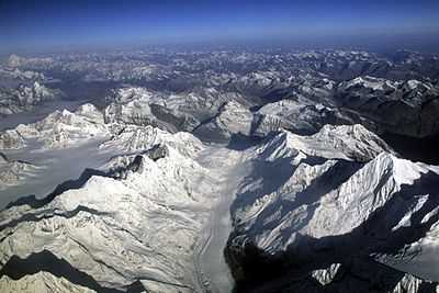
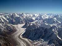
The Baltoro Glacier in the Karakoram, Baltistan, Northern Pakistan, in the image on the lower right, at 62 kilometres (39 mi) in length, is one of the longest alpine glaciers on Earth.
Emissions
Def. a "thick, floating platform of ice that forms where a glacier or ice sheet flows down to a coastline and onto the ocean surface"[38] is called an ice shelf.
"Ice shelves are permanent floating sheets of ice that connect to a landmass."[39]
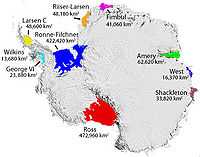
"Most of the world's ice shelves hug the coast of Antarctica [as shown in the image on the right]. However, ice shelves can also form wherever ice flows from land into cold ocean waters, including some glaciers in the Northern Hemisphere. The northern coast of Canada's Ellesmere Island is home to several well-known ice shelves, among them the Markham and the Ward Hunt ice shelves."[39]
"Ice from enormous ice sheets slowly oozes into the sea through glaciers and ice streams. If the ocean is cold enough, [...] newly arrived ice doesn't melt right away. Instead it may float on the surface and grow larger as glacial ice behind it continues to flow into the sea. Along protected coastlines, the resulting ice shelves can survive for thousands of years, bolstered by the rock of peninsulas and islands. Ice shelves grow when they gain ice from land, and occasionally shrink when icebergs calve off their edges."[39]
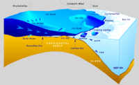
The schematic on the right presents glaciological and oceanographic processes along the Antarctic coast. Snow falling in the accumulation zone creates an upstream stress. The ice shelf has built up to a thickness of about 4 km. The ice flows along the glacier and in ice streams within. On the coast the ice loses contact with its bedrock at the grounding line and becomes significantly thinner by some 100 m. It forms an ice shelf over the continental shelf. At the edge of the continental shelf, tabular icebergs calve.
"Satellite imagery [third image on the right] revealed that the western front of the 13,680 square kilometer (5,282 square mile) Wilkins Ice Shelf began to collapse because of rapid climate change in a fast-warming region of Antarctica."[39]
"This satellite image [fourth on the right] shows floating chunks of ice from the 2008 Wilkins Ice Shelf collapse."[39]
"Most ice shelves are fed by inland glaciers. Together, an ice shelf and the glaciers feeding it can form a stable system, with the forces of outflow and back pressure balanced. Warmer temperatures can destabilize this system by increasing glacier flow speed and—more dramatically—by disintegrating the ice shelf. Without a shelf to slow its speed, the glacier accelerates. After the 2002 Larsen B Ice Shelf disintegration, nearby glaciers in the Antarctic Peninsula accelerated up to eight times their original speed over the next 18 months. Similar losses of ice tongues in Greenland have caused speed-ups of two to three times the flow rate in just one year."[39]
"Ice shelves fall into three categories: (1) ice shelves fed by glaciers, (2) ice shelves created by sea ice, and (3) composite ice shelves (Jeffries 2002). Most of the world's ice shelves, including the largest, are fed by glaciers and are located in Greenland and Antarctica."[39]
Meteors
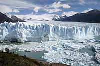
The image on the right shows calving by the Perito Moreno Glacier, in Los Glaciares National Park, southern Argentina.
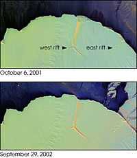
"Calving of huge, tabular icebergs is unique to Antarctica, and the process can take a decade or longer. Calving results from rifts that reach across the shelf. In the case of Antarctica's Amery Ice Shelf, the calving area resembles a loose tooth [images on the second right]."[40]
"On a stable ice shelf, calving is a near-cyclical, repetitive process producing large icebergs every few decades. The icebergs drift generally westward around the continent, and as long as they remain in the cold, near-coastline water, they can survive decades or more. However, they eventually are caught up in north-drifting currents where they melt and break apart."[40]
"In Greenland, floating ice tongues downstream from large outlet glaciers are more broken up by crevasses. Calving of the ice tongues releases armadas of smaller, steep-sided icebergs that drift south sometimes reaching North Atlantic shipping lanes. Calving of the large glacier, Jacobshavn, on the east coast of Greenland is responsible for the majority of icebergs reaching Atlantic shipping and fishing areas off of Newfoundland and most likely shed the iceberg responsible for the sinking of the Titanic in 1912. The Petermann Glacier in northwestern Greenland also shed a large ice island in August 2010. These denizens of the ocean are now tracked by the National Ice Center in the United States, along with other organizations."[40]
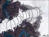
"By 2006, the Jacobshavn Glacier [third image on the right] had retreated back to where its two main tributaries join, leading to two fast-flowing glaciers where there had previously been just one."[40]
"The rapidly retreating Jakobshavn Glacier in western Greenland drains the central ice sheet. This image [third one on the right] shows the glacier in 2001, flowing from upper right to lower left. Terminus locations before 2001 were determined by surveys and more recent contours were derived from Landsat data. The recent stages of retreat have widened the ice front, placing more of the glacier in contact with the ocean."[40]
"In recent years, calving of the largest ice tongues in Greenland (in particular, Jacobshavn, Helheim, and Kangerdlugssuaq) has accelerated probably due to warmer air and/or ocean temperatures. As the ice tongues have retreated, the reduced backpressure against the glacier has allowed these glaciers to accelerate significantly."[40]
"The images [fourth set of images on the right] show a tabular iceberg calving from an ice shelf. This iceberg happens to be calving from the remnant piece of the Larsen B ice shelf at the southwestern corner of the embayment. While the Larsen B Ice Shelf underwent disintegration [...], this was a normal calving event."[40]
"Large tabular iceberg calvings are natural events that occur under stable climatic conditions, so they are not a good indicator of warming or changing climate. Over the past several decades, however, meteorological records have revealed atmospheric warming on the Antarctic Peninsula, and the northernmost ice shelves on the peninsula have retreated dramatically (Vaughan and Doake 1996)."[40]
"The most pronounced ice shelf retreat has occurred on the Larsen Ice Shelf, located on the eastern side of the Antarctic Peninsula's northern tip. The shelf is divided into four regions from north to south: A, B, C, and D."[40]
Gamma rays
"Airborne gamma ray spectrometry data provide information about the distribution of potassium (K), equivalent uranium (eU), and equivalent thorium (eTh) in the upper 1 m of surficial materials [...] Knowledge of the distribution of surface materials is useful for interpreting gamma ray data because gamma radiation is attenuated by water and unconsolidated sediments [...] Ratio patterns of K, eU, and eTh in surficial materials can enhance subtle variations in the elemental concentrations caused by lithological variation of the alteration processes associated with mineralization."[41]
Visuals
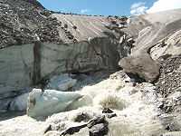
At the mouth of Schlatenkees glacier, in the image on the right, water comes rushing out along with sediment that alters the color of the ice and the water.
Blues

Even when a grotto forms underneath a glacier, the ice still exhibits its typical blue color as with the Perito Moreno Glacier, in Los Glaciares National Park, southern Argentina, in the image on the right.
"Majestic glaciers and thick snow banks act like filters that absorb red light, making a crevasse or deep hole appear blue."[42]
Cyans
"Blue to blue-green hues are scattered back when light deeply penetrates frozen waterfalls and glaciers."[42]
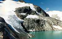
"Glacier Flour causes the blue green color in this Lake on Mt. Daniels. The flour is clay sized particle resulting from the glacier eroding the rock at its base."[36]
Oranges
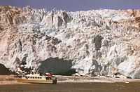
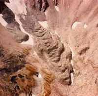
The color of the sediment deposited on or scraped away from the confining rocks often colors a glacier and its meltwater. Here it does so to the Holgate Glacier imaged on the right.
Radars
"One example of an ice shelf composed of compacted, thickened sea ice is the Ward Hunt Ice Shelf off the coast of Ellesmere Island in northern Canada. Canadian RADARSAT image shows the shelf in August 2002, when a crack made its way down the length of the shelf."[39]
The image on the left is a Radarsat portrayal of ice streams flowing into the Filchner-Ronne Ice Shelf. This image uses data from the Radarsat RAMP 125m Mosaic. The dataset is freely available from the National Snow and Ice Data Center.
Gaseous objects
At some altitudes when warm, moist air comes in contact with a glacier, water vapor condenses and forms fog as imaged on the right on the Gorner Glacier in Switzerland.
The "firn air analyses of Site M in Dronning Maud Land, Antarctica (15°E, 75°S, 3453 m.a.s.l) are described. These firn air analyses were measured with gas chromatography, yielding concentration profiles with depth for a wide variety of trace gases."[9]
The "firn air analyses are focussed on the non-methane hydrocarbons (NMHCs): ethane, propane and acetylene, and methyl chloride. The NMHCs were studied because very little is known about their long-term and seasonal trend in the atmosphere around Antarctica and Southern Hemisphere in general whereas these NMHCs play an important role in the atmospheric oxidation chemistry. Studying the long-term and seasonal trend for methyl chloride is very interesting because this gas shows a large spatial variability although this is not expected because of its large lifetime."[9]
The "location and age of the oldest firn air, being 156±22 years for the mean age of CO2 at pore close-off depth at 82°E, 83°S on the Antarctic plateau."[9]
The "chemical signature based on 16 trace elements, a chemical fingerprint, of an unknown 1500-year old volcanic horizon is measured with inductively coupled plasma mass spectrometry (ICP-MS). [The] trace metal chemistry is compared to the DEP record directly measured in the field. With the chemical fingerprint for the 1500-year old volcanic horizon, which has been scaled and normalised to allow comparison among various geochemical data, Mount Erebus is identified as a good candidate for the source."[9]
Below the firn is a zone in which seasonal layers alternately have open and closed porosity. These layers are sealed with respect to diffusion. Gas ages increase rapidly with depth in these layers. Various gases are fractionated while bubbles are trapped where firn is converted to ice.[43]
The surface layer is snow in various forms, with air gaps between snowflakes. As snow continues to accumulate, the buried snow is compressed and forms firn, a grainy material with a texture similar to granulated sugar. Air gaps remain, and some circulation of air continues. As snow accumulates above, the firn continues to densify, and at some point the pores close off and the air is trapped. Because the air continues to circulate until then, the ice age and the age of the gas enclosed are not the same, and may differ by hundreds of years. The gas age–ice age difference is as great as 7 kyr in glacial ice from Vostok.[44]
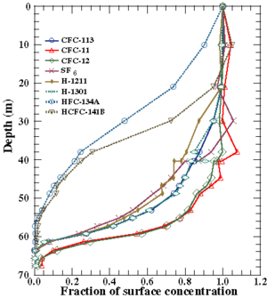
Gases involved in ozone depletion, CFCs, chlorocarbons, and bromocarbons, were measured in firn and levels were almost zero at around 1880 except for CH3Br, which is known to have natural sources.[45]
Similar study of Greenland firn found that CFCs vanished at a depth of 69 m (CO2 age of 1929).[46]
Analysis of the Upper Fremont Glacier ice core showed large levels of chlorine-36 that definitely correspond to the production of that isotope during atmospheric testing of nuclear weapons. This result is interesting because the signal exists despite being on a glacier and undergoing the effects of thawing, refreezing, and associated meltwater percolation.[47]
36Cl has also been detected in the Dye-3 ice core (Greenland)[48], and in firn at Vostok.[49]
Studies of gases in firn often involve estimates of changes in gases due to physical processes such as diffusion. However, it has been noted that there also are populations of bacteria in surface snow and firn at the South Pole, although this study has been challenged.[50][51]
It had previously been pointed out that anomalies in some trace gases may be explained as due to accumulation of in-situ metabolic trace gas byproducts.[52]
Liquid objects
Def. "(1) a large outburst flood that usually occurs when a glacially dammed lake drains catastrophically (2) any catastrophic release of water from a glacier"[2] is called a jokulhlaup.
"Proglacial stream water is a mixture of supraglacial and subglacial meltwater with groundwater inputs (Raiswell 1984). The term supraglacial is used for both superglacial (surface melt) and englacial (throughput) meltwaters that do not come into contact with subglacial water until just before or after the portal of the glacial stream. Subglacial meltwaters are characterized by high suspended and dissolved solids and residence times on the order of several days, while supraglacial meltwaters are typically characterized by very low dissolved and suspended solids, atmospheric pCO2 levels (10-3.5 atm), and residence times of < 24 h (Raiswell 1984). Collins (1979) found that supraglacial meltwater accounted for a large percentage (50-80%) of the total meltwater discharge of two alpine glaciers during warm summer months. Mixing of very dilute supraglacial meltwaters with subglacial water rich in finely ground glacial flour creates a reactive environment for ion exchange (Lemmens and Roger 1978) and mineral dissolution (Raiswell1984). An enhanced reactivity of minerals in glacial flour due to small particle size has been proposed frequently (e.g. Reynolds and Johnson 1972; Raiswell 1984) and has been qualitatively simulated in the laboratory (Keller and Reesman 1963)."[53]
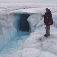
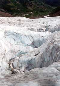
"A moulin is a narrow, tubular shaft in a glacier that provides a pathway for water to travel from the glacier's surface to its bottom. [Alberto] Behar and co-investigator Dr. Konrad Steffen of the University of Colorado, Boulder, led an expedition to send a JPL-built probe down into these glacial chutes in the remote and isolated Pakisoq region of the West Greenland Ice Sheet. That dynamic area of Earth's northern polar region is not well understood and is responding rapidly to climate change. Previous NASA measurements there using global positioning system data show the ice there moves an average of about 20 centimeters (8 inches) a day, accelerating to about 35 centimeters (14 inches) a day during the summer melt. The scientists set out to see if these moulins, or pathways, within and beneath these mountains of ice can shed new light on how glacial water flows from the ice sheet to the sea."[54]
"How water is distributed within a glacier and the rate at which it permeates through to a glacier's bottom affects the glacier's ability to store water, its pressure, and the speed at which a glacier moves. Scientists have long known that ponds of melted ice on the surfaces of glaciers and the moulins they create allow glaciers to flow faster. Our study -- the first of its kind in this region -- we hope will provide a better understanding of the factors at work here."[55]
"In glaciological terms, moulins (French for "mill") are essentially vertical "rivers" that serve as a glacier's internal plumbing system, carrying water out of the glacier from melt water lakes on the surface. They can be hundreds of meters deep and up to 10 meters (33 feet) wide. The melt water lakes are typically found in the undulations of the ice sheet all around Greenland between 500 and 1,500 meters (1,640 to 4,920 feet) above sea level. Occasionally, the lower end of a moulin may be exposed in the face of a glacier."[54]
"In Greenland, the surface of the ice sheet moves at varying speeds, on both seasonal and shorter-term time scales. Seasonally, glacial water penetrates to the glacier bed through significant thicknesses of cold ice. Occasionally, however, there are periods when water flows rapidly into glacial drainage systems. For example, early in the melt season, new drainage connections are established between glacial surfaces and their beds, resulting in sudden new flows of water out of the glaciers. In the middle of the melt season, surface melting resumes after periods of cold weather, which can partially close sub-glacial channels."[54]
"Once the probe descended to 110 meters (361 feet), it encountered horizontally flowing water and debris about one to two meters (3.3 to 6.6 feet) deep. In this particular moulin, the water flows out in well-developed channels to the edge of the ice sheet. At the time of the experiment, the scientists measured the water flow rate of the surface melt rivers feeding the moulin at approximately 15 cubic meters a second (about 238,000 gallons a minute)."[54]
"Video data from the probe revealed enormous ice caverns formed by the moulin deep beneath the glacial surface. This particular moulin appears to fill up with snow, which hardens during the winter. When the surface melts in the summer, this ice forms snow bridges."[54]
Hydrology
Def. "the melt from the entire glacier"[36] is called glacier runoff.
"It is highest on warm dry days when runoff from other sources is at its lowest."[36]
Def. "a lake beyond the terminus of a glacier"[36] is called a proglacial lake.
Def. a stream running on top of a glacier or cutting a channel into a glacier from the top is called a supraglacial stream.[36]
"Almost every general textbook on hydrology includes a chapter on snow: measurement, melting, calculation of snowmelt runoff, and forecasting of snowmelt floods."[56]
Measurement "of glacier growth and wastage, predicting glacier runoff, the buffering effect of glaciers on streamflow variations, glacier outburst floods, or the internal structure and hydraulic properties of glaciers [are how] glacier hydrology differs, both qualitatively and quantitatively, from the hydrology of conventional streams and even the hydrology of snow. Yet about three-fourths of all the freshwater on the earth is temporarily detained as glacier ice (equivalent to the world's precipitation for about 60 years), and in many parts of the world hydroelectric, irrigation, and domestic water resources are directly dependent on glacier runoff."[56]
"Hydrologically, perhaps the most significant aspect is that when the glacier is in the process of adjusting to climate change (this occurs continually because climate changes quickly and glaciers slowly), precipitation is being stored or released from storage [3]. Not everyone is aware that, during the 1920-45 period when many runoff "base" or "normal" periods are defined, glaciers in most populated parts of the world were receding and releasing streamflow greatly in excess of precipitation [4]."[56]
"Mountain snow cover is a critical resource as these high elevation mountain regions provide the majority of fresh water supply in arid and semi-arid environments to more than a billion of the Earth’s population [Bales et al., 2006]. The duration of snow pack in mountain regions critically controls the timing and magnitude of water supplies, power generation, agriculture timing, and forest fire regimes [Westerling et al., 2006], as well as the duration over which glacial ice is exposed to absorption and enhanced ablation. Some studies already suggest that climate change has induced earlier snowmelt-fed runoff [Mote, 2003; Stewart et al., 2005]."[57]
Earlier "snowmelt and its effects on mountain water resources and glacial extent is a likely scenario in many of the world’s mountain ranges under enhanced dust deposition."[57]
Rocky objects
Def. "looks like a mountain glacier and has active flow; usually includes a poorly sorted mess of rocks and fine material; may include: (1) interstitial ice a meter or so below the surface (ice-cemented), (2) a buried core of ice (ice-cored), and/or (3) rock debris from avalanching snow and rock"[2] is called a rock glacier.
At the right, "Frying Pan Glacier, Colorado, is almost entirely covered by rocks and debris in this photograph from 1966."[2]
Ice-rafted debris
"Correlations between North Atlantic marine sequences and Greenland ice-core δ 18O records showed that high amounts of ice-rafted debris (IRD) and extremely cold [sea surface temperatures] SSTs occurred prior to GIS 12, 8, 4, 2 and 1 (Bond et al. 1993). These so-called Heinrich events [in the diagram of the Bølling section], which originated from surges of Northern Hemisphere ice sheets (Hemming 2004), caused a rise in global sea level (Chappell 2002; Lambeck et al. 2002; Rohling et al. 2004; Rohling & Pälike 2005), which in turn could have caused further destabilization of the large ice sheets. Provenance analyses of Heinrich-layer detritus in North Atlantic marine sediments indicate that the IRD is derived from the Hudson Strait region/Laurentide ice sheet (Hemming 2004), although precursor events could possibly have originated from European and Icelandic ice sheets (Grousset et al. 2000, 2001)."[28]
Moraines
"Lateral and terminal moraines of a valley glacier, Bylot Island, Canada [are shown in the image at the left]. The glacier formed a massive sharp-crested lateral moraine at the maximum of its expansion during the Little Ice Age. The more rounded terminal moraine at the front consists of medial moraines that were created by the junction of tributary glaciers upstream."[2]
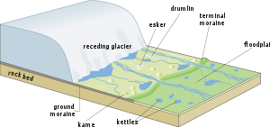
Features of a glacial landscape
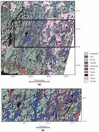
In the two images on the right, (a) is a predictive "surficial geology map based on Landsat TM. [The outline of an area] covered by the traditional surficial geology map is shown [outlined by] a black line. (b) [is the traditional] surficial geology map, based on 1:50,000-scale field mapping and aerial photograph interpretations".[41]
Trimlines
Def. a "clear boundary line on the wall of a glacier valley that delineates the maximum recent thickness of a glacier"[58] is called a trimline.
Isostasy
Def. the "state of balance or pressure equilibrium thought to exist within the Earth's crust, whereby the upper lithosphere floats on denser magma beneath"[59] is called isostasy.
"It's probably no accident that two of the largest epicontinental seas (seas extending deep into the continent) on Earth are Hudson Bay and the Baltic, both dead center in areas of active isostatic uplift. In all likelihood, the crust in these regions is still depressed and has not finished rising, and when uplift is complete both seas will mostly or entirely disappear. Gravity measurements suggest that the crust in the Hudson Bay region has another 100 meters still to rise."[60]
Oxygens
Many rocky objects are composed of oxide minerals. Oxygen has three known stable isotopes: 16O, 17O, and 18O.
"The stable isotopic compositions of low-mass (light) elements such as oxygen, hydrogen, [helium, lithium, beryllium, boron,] carbon, nitrogen, [fluorine, neon, sodium, magnesium, aluminum, silicon, phosphorus,] and sulfur are normally reported as "delta" ([δ]) values in parts per thousand (denoted as ‰ [per mille]) enrichments or depletions relative to a standard of known composition."[61]
For 18O to 16O:
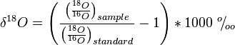
The "ratio [by convention is] of the heavy to light isotope in the sample or standard."[61]
"Various isotope standards are used for reporting isotopic compositions; the compositions of each of the standards have been defined as 0‰. Stable oxygen and hydrogen isotopic ratios are normally reported relative to the SMOW standard ("Standard Mean Ocean Water" (Craig, 1961b)) or the virtually equivalent VSMOW (Vienna-SMOW) standard. Carbon stable isotope ratios are reported relative to the PDB (for Pee Dee Belemnite) or the equivalent VPDB (Vienna PDB) standard. The oxygen stable isotope ratios of carbonates are commonly reported relative to PDB or VPDB, also. Sulfur and nitrogen isotopes are reported relative to CDT (for Cañon Diablo Troilite) and AIR (for atmospheric air), respectively."[61]
Spectrometers
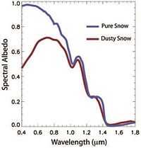
"Snow has the highest albedo of any naturally occurring surface on Earth. However, when impurities such as dust or soot are present, snow albedo decreases (particularly in visible wavelengths) [Conway et al., 1996; Warren and Wiscombe, 1980] [Figure at right]. With enhanced absorption by dust, grain growth rates increase and further depress snow albedo. Dust has high potential to sustain shortwave radiative forcing after deposition because particles tend to accumulate near the snow surface as ablation advances [Conway et al., 1996]. Deposition in mountain ranges comes primarily in the spring when frontal systems entrain dust particles from disturbed and loose soils [Wake and Mayewski, 1994], coinciding with solar irradiance approaching its annual maximum."[57]
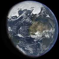
Earth
Earth has ice sheets, ice caps, ice fields, and glaciers.
Greenland ice sheet petrognosy
1.jpg)

Def. the study of the structure of rocky objects, or rocks, is called petrognosy.
Sea ices
Def. "frozen ocean water"[39] is called sea ice.
"It forms, grows, and melts in the ocean."[39]
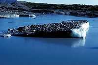
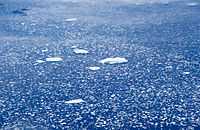
Def. a "large consolidated mass of floating sea ice"[62] is called pack ice.
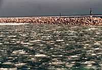
Pack ice in the image on the right is drifting southward in the East Greenland current during July 1996.
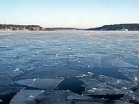
Drift ices
Def. one "or more floating slabs of ice which have become detached from larger sheets or shoreline glaciers and which are moved by wind or sea currents"[63] is called drift ice.
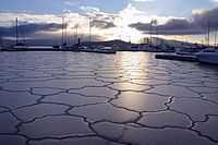
Def. "a form of ice that forms on water covered to some degree in slush"[64] is called pancake ice.
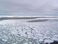
In the first image on the left, when "waves buffet the freezing ocean surface, characteristic "pancake" sea ice forms."[65]
"Sheets of sea ice form when frazil crystals float to the surface, accummulate and bond together. Depending upon the climatic conditions, sheets can develop from grease and congelation ice, or from pancake ice."[66]
"If the ocean is rough, the frazil crystals accummulate into slushy circular disks, called pancakes or pancake ice, because of their shape. A signature feature of pancake ice is raised edges or ridges on the perimeter, caused by the pancakes bumping into each other from the ocean waves. If the motion is strong enough, rafting occurs. If the ice is thick enough, ridging occurs, where the sea ice bends or fractures and piles on top of itself, forming lines of ridges on the surface. Each ridge has a corresponding structure, called a keel, that forms on the underside of the ice. Particularly in the Arctic, ridges up to 20 meters (60 feet) thick can form when thick ice deforms. Eventually, the pancakes cement together and consolidate into a coherent ice sheet. Unlike the congelation process, sheet ice formed from consolidated pancakes has a rough bottom surface."[66]
Locations on Earth
"The coordinates should describe the location of a glacier as accurately as possible. In the former [World Glacier Inventory] WGI it was recommended to place this point in the upper part of the ablation area near the centre of the main stream. This recommendation is still valid for manual assignment of the coordinates. Considering the available GIS-based methods, it is also acceptable to create a label point inside a glacier polygon automatically, and add the x-y coordinates of this point to the attribute table of the respective glacier".[67]
"In regions where glacier changes are small and the coordinates from a former glacier inventory are available, it should be determined whether the former coordinates are still within the current outlines. If they have been stored with a sufficient number of digits, it is possible that only a few label points have to be shifted slightly. This way of assigning label points is preferable in order to establish a link to the former inventory."[67]
"Highest, mean and lowest glacier elevation are also basic entries in the former WGI. It is recommended that they be derived from glacier-specific statistical analysis using the elevation information from the [digital terrain model] DTM and a local glacier ID as an identifier for the respective glacier or zone."[67]
"The aspect or orientation of a glacier is a useful parameter for all kinds of modelling (e.g. Evans, 2006). In the former UNESCO guidelines this variable was restricted to eight directions: ‘Orientation of the down-glacier direction ac- cording to the eight cardinal points ... should be given.’ The mean aspect as derived from a DTM allows one to consider the value of all individual cells covered by the glacier and to derive a mean value in the full 0–3608 range. It must be taken into account that aspect is a circular parameter, which means that mean values must be derived by a decomposition in the respective sine and cosine values (Paul, 2007; Manley, 2008)."[67]
Def. the "data present in contour lines; measurement of altitude or depth versus area"[68] is called hypsography.
Def. the "measurement of elevation relative to sea level"[69] is called hypsometry.
Stratigraphy
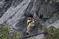
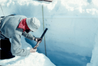
Glaciology like many fields within geology often requires field work.
The image at right shows a glaciologist taking a sample of a melting permafrost outcropping.
The second image at the right shows sampling of the Taku Glacier surface in Alaska. Such sampling demonstrates that there is increasingly denser firn between surface snow and blue glacier ice.
Glacial physics
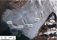
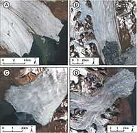

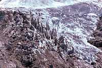
"Glacier length is the most demanding parameter regarding additional manual work and uncertainty."[67]
"The definitions used in the former guide are:"[67]
Def. the "average of the lengths of each tributary along its longest flowlines to the glacier snout"[67] is called the mean length.
Def. the "longest flowline of the whole glacier"[67] is called the maximum length.
"When a DTM of sufficient quality is available, automated techniques can be used to identify the highest glacier point and then follow the steepest downward gradient until the curvature of the glacier surface changes from concave to convex. In this region – in general, the ablation area – manual digitization close to the central flowline of the main trunk might be more efficient. For manual digitization of the length, the flowline should cross elevation contours perpendicularly. Uncertainty of the result is thereby reduced if flowline digitization starts at the lower end of the glacier."[67]
Large apparently solid objects of ice flow. Gravity is a likely force acting on large solid ice objects. Many glaciers slide over their beds. Ice "itself can flow like a very viscous fluid, [...] increases in velocity after heavy rain [...] showed that water helps a glacier to slide. [...] the velocity is greatest in the central part and decreases progressively toward each side. [...] a glacier moves more slowly near its head and terminus than elsewhere. [...] velocity vectors do not parallel the glacier surface; relative to the surface, they are inclined slightly downward in the higher parts of the glacier, where snow accumulates, and slightly upward in the lower reaches to compensate for ice lost by melting."[35]
Ice "moves more rapidly at the surface than at depth. [...] in general, although slow across-glacier extrusion flow sometimes occurs in narrow valleys."[35]
There is a "time lag between the advance of the terminus and the increase in snowfall that produced it."[35]
"Mean slope is a value that could be derived from elevation range and glacier length and was thus not listed in the guidelines by UNESCO/IASH (1970). Mean slope as derived for each glacier from the DTM with zone statistics is independent of the glacier length and refers to all individual cells of the DTM (Manley, 2008). [Mean] slope is a good proxy for other parameters like mean thickness (Haeberli and Hoelzle, 1995) [...] A large number of further parameters characterizing individual glaciers (e.g. driving stress, slope-dependent thick- ness, volume, thermal conditions, response and reaction times) can be derived or estimated from the basic parameters".[67]
"Annual flow velocities on the Austre Torellbreen tongue [are] derived from displacement of crevasses on a pair of ASTER images (2005 and 2006) [in the image at right]: black lines – location of crevasses in 2005, white lines – location of crevasses in 2006, blue line – front position in 2005. The background image is a portion of the FCC of ASTER scene (acquired on 23.07.2006)."[70]
The mean flow velocity of the Svalbard tidewater glacier Austre Torellbreen is 260 m yr-1.[70]
"Examples of ASTER geocoded images (321 bands) of glaciers [in the second image on the right are] classified into different groups of flow dynamics: a) Negribreen – very slow or stagnant glacier (5.08.2003) [date surveyed 05 August 2003 at a mean flow velocity of <30 m yr-1]; b) Storbreen – slow−flowing glacier (7.08.2004) [80 m yr-1]; c) Austre Torellbreen – fast−flowing glacier (23.07.2005) [260 m yr-1]; [and] d) Perseibreen – active surge glacier (7.08.2004) [730-910 m yr-1]."[70]
Def. "a glacier that is not moving significantly, notice lack of crevassing"[36] is called a stagnant glacier.
Def. a glacier that is
- "moving at reasonable [a] pace",[36]
- "has crevassing",[36] and
- "is eroding its bed"[36] is called an active glacier.
When the stress of the layer above exceeds the inter-layer binding strength, it moves faster than the layer below.[15]
The geothermal heat flux becomes more important the thicker a glacier becomes.[16]
Ice streams
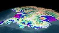
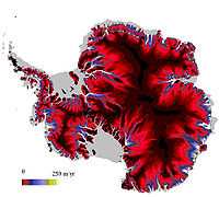
The image on the right shows animated motions of ice flowing across Antarctica.
The second image on the right shows the ice stream velocities of Antarctic ice from zero (black) up to 250m/yr (cream white).
"Although they account for only 10% of the volume of the ice sheet, ice streams are sizeable features, up to 50 km wide, 2000 m thick and hundreds of km long. Some flow at speeds of over 1000 m per year and most of the ice leaving the ice sheet passes through them."[71]
"Ice streams generally form where water is present, but other factors also control their velocity, in particular whether the ice stream rests on hard rock or soft, deformable sediments. At the edges of ice streams deformation causes ice to recrystallise making it softer and concentrating the deformation into narrow bands or shear margins. Crevasses, cracks in the ice, result from rapid deformation and are common in shear margins."[71]
Fracture zones
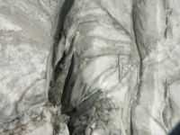
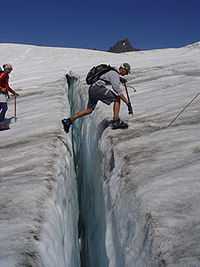
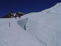
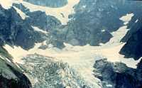
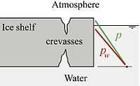
Shear or herring-bone crevasses on the Emmons Glacier shown on the right often form near the edge of a glacier where interactions with underlying or marginal rock impede flow. In this case, the impediment appears to be some distance from the near margin of the glacier.
Ice cracks are also imaged in the Titlis Glacier shown on the second right.
In the third image on the right, a graduate student crosses a crevasse on the Easton Glacier, Mount Baker, in the North Cascades of the United States.
The fourth image on the right shows a crevasse on the Easton Glacier.
"Glacier mass balance is assessed in crevasses such as this on Easton Glacier. Note the horizontal horizon marking the 2007 summer surface with 3.2 m of 2008 winter snowpack on top."[36]
"Crevasses [o]pen because of an acceleration of the glacier."[36]
Def. "an area of rapid movement on a steep slope with extensive open crevassing"[36] is called an icefall.
The "ice in the immediate vicinity of the shelf front is being weakened due to accumulating fractures (which may be transported from further inland), which finally leads to calving events. This calls for the incorporation of some kind of damage or fracture parameterization into ice-shelf models, in order to predict/assess their stability and possible onsetting instabilities, which have been shown to fall apart on a surprisingly short timescale."[72]
"The great unsolved problem in ice-shelf dynamics (perhaps in the whole of glaciology) is the treatment of the shelf front."[72]
"No response of an ice-sheet/ice-shelf system to climate variations can be computationally forecasted, unless this boundary condition is properly parameterized."[73]
"Dynamically, an equivalent description of the calving rate – the second condition – is the relevant climatological statement, describing the mass loss of the shelf, for which only first estimates exist ... The difficulty with parameterizations of the calving rate is its inter- mittent non-smooth occurrence in nature. Such discon- tinuous behavior of the mass loss by ice shelves is most likely not adequately parameterizable, but smeared over long time scales (of decades) a smooth parameterization may well be possible".[73]
"[A]long-flow ice shelf spreading [may be] the dominant control on calving".[74]
The "influence of water penetrating into any crack which opens at the base of the ice shelf [is] at a pressure close to the ice overburden pressure[. It] tends to counterbalance the action of the latter as an effect opposing crack opening."

where  is the water pressure at a given depth [in the figure on the left]. This change accounts for the fact that the water pressure reduces the contribution to failure of the local mean pressure in ice near the base of the ice shelf that is exposed to crevasses. It assures that damage evolution in an ice shelf always starts at the top or base, not somewhere in between."[72]
Technology
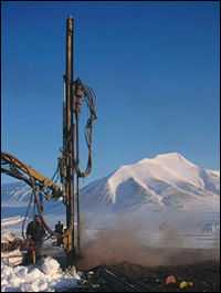
"Satellite imagery and data from ground surveys are used to reconstruct the integrated pattern of the principal longitudinal and transverse features produced on a continent-wide scale by the last ice sheets in Europe and North America."[75]
"Boreholes [made by rigs like that imaged at the right] in Svalbard, Norway, for example, indicate that ground temperatures rose 0.4C over the past decade, four times faster than they did in the previous century".[76]
Research
Hypothesis:
- Glaciers have occurred throughout Earth history.
Control groups

The findings demonstrate a statistically systematic change from the status quo or the control group.
“In the design of experiments, treatments [or special properties or characteristics] are applied to [or observed in] experimental units in the treatment group(s).[77] In comparative experiments, members of the complementary group, the control group, receive either no treatment or a standard treatment.[78]"[79]
Proof of concept
Def. a “short and/or incomplete realization of a certain method or idea to demonstrate its feasibility"[80] is called a proof of concept.
Def. evidence that demonstrates that a concept is possible is called proof of concept.
The proof-of-concept structure consists of
- background,
- procedures,
- findings, and
- interpretation.[81]
See also
References
- 1 2 Jane Qiu (01 October 2014). "Tibetan plateau gets wired up for monsoon prediction". Nature.com. Retrieved 2014-10-02.
- 1 2 3 4 5 6 7 8 9 10 11 Janet Beitler (2014). "Cryosphere Glossary". National Snow and Ice Data Center. Retrieved 2014-09-20.
- ↑ Robert Gilbert, Niels Nielsen, Henrik Möller, Joseph R. Desloges, and Morten Rasch (2002). "Glacimarine sedimentation in Kangerdluk (Disko Fjord), West Greenland, in response to a surging glacier". Marine Geology 191: 1-18. http://geog.queensu.ca/gilbert/surge%20paper.PDF. Retrieved 2014-09-24.
- 1 2 3 4 5 Nicholas J. Shackleton, Maria Fernanda Sánchez-Goñi, Delphine Pailler, and Yves Lancelot (2003). "Marine Isotope Substage 5e and the Eemian Interglacial". Global and Planetary Change 36: 151-5. doi:10.1016/S0921-8181(02)00181-9. http://www.colorado.edu/geography/class_homepages/geog_5241_f09/media/Readings/shackletonetal.pdf. Retrieved 2014-10-11.
- ↑ Harvey, Eveline (14 January 2011). "NZ blue ice sighting an unexpected treat for tourists". The New Zealand Herald. Retrieved 21 September 2011.
- ↑ Why Is Water Blue
- ↑ "Blue ice (glacial)". Wikipedia (San Francisco, California: Wikimedia Foundation, Inc). March 29, 2013. http://en.wikipedia.org/wiki/Blue_ice_(glacial). Retrieved 2013-05-29.
- 1 2 3 4 5 6 7 8 9 10 11 12 13 14 15 16 17 18 19 20 21 22 23 Willi Dansgaard (2005). The Department of Geophysics of The Niels Bohr Institute for Astronomy, Physics and Geophysics at The University of Copenhagen, Denmark. ed. Frozen Annals Greenland Ice Cap Research. Copenhagen, Denmark: Niels Bohr Institute. pp. 123. ISBN 87-990078-0-0. http://www.iceandclimate.nbi.ku.dk/publications/FrozenAnnals.pdf/. Retrieved 2014-10-05.
- 1 2 3 4 5 Karsten Adriaan Kaspers (04 October 2004). "Chemical and physical analyses of firn and firn air: from Dronning Maud Land, Antarctica; 2004-10-04". Utrecht, Netherlands: University of Utrecht. Retrieved October 14, 2005.
- 1 2 3 Jan-Gunnar Winther (June 1993). "Landsat TM derived and in situ summer reflectance of glaciers in Svalbard". Polar Research 12 (1): 37-55. doi:10.1111/j.1751-8369.1993.tb00421.x. http://www.polarresearch.net/index.php/polar/article/download/6702/7535. Retrieved 2014-09-27.
- 1 2 "ice field, In: Wiktionary". San Francisco, California: Wikimedia Foundation, Inc. 20 September 2014. Retrieved 2014-10-09.
- ↑ "aufeis, In: Wiktionary". San Francisco, California: Wikimedia Foundation, Inc. 16 November 2014. Retrieved 2014-11-25.
- ↑ "naled, In: Wiktionary". San Francisco, California: Wikimedia Foundation, Inc. 16 November 2014. Retrieved 2014-11-25.
- 1 2 Gifford H Miller, Aslaug Geirsdottir, Yafang Zhong, Darren J Larsen, Bette L Otto-Bliesner, Marika M Holland, David Anthony Bailey, Kurt A. Refsnider, Scott J. Lehman, John R. Southon, Chance Anderson, Helgi Björnsson, and Thorvaldur Thordarson (January 2012). "Abrupt onset of the Little Ice Age triggered by volcanism and sustained by sea-ice/ocean feedbacks". Geophysical Research Letters 39 (2): L02708. doi:10.1029/2011GL050168. http://adsabs.harvard.edu/abs/2012GeoRL..39.2708M. Retrieved 2014-10-09.
- 1 2 A. Speranza, J. van der Plicht, and B. van Geel (November 2000). "Improving the time control of the Subboreal/Subatlantic transition in a Czech peat sequence by 14C wiggle-matching". Quaternary Science Reviews 19 (16): 1589-1604. doi:10.1016/S0277-3791(99)00108-0. http://www.researchgate.net/publication/30494985_Improving_the_time_control_of_the_SubborealSubatlantic_transition_in_a_Czech_peat_sequence_by_14C_wiggle-matching/file/60b7d51c350cf2efa0.pdf. Retrieved 2014-11-04.
- 1 2 E.B. Karabanov, A.A. Prokopenko, D.F. Williams, and G.K. Khursevich (March 2000). "A new record of Holocene climate change from the bottom sediments of Lake Baikal". Palaeogeography, Palaeoclimatology, Palaeoecology 156 (3-4): 211–24. doi:10.1016/S0031-0182(99)00141-8. http://www.sciencedirect.com/science/article/pii/S0031018299001418. Retrieved 2014-11-04.
- 1 2 3 4 5 6 J. W. Franks and W. Pennington (April 1961). "The Late-Glacial and Post-Glacial Deposits of the Esthwaite Basin, North Lancashire". New Phytologist 60 (1): 27-42. http://onlinelibrary.wiley.com/store/10.1111/j.1469-8137.1961.tb06237.x/asset/j.1469-8137.1961.tb06237.x.pdf;jsessionid=EB6966DF0A2FBCC3534CCD6A6413808D.f02t01?v=1&t=i23es9k1&s=e619673cf5bc8be51450a303a914df03f8cba94d. Retrieved 2014-11-04.
- ↑ J. H. Mercer (October 1967). "Glacier resurgence at the Atlantic/sub-Boreal transition". Quarterly Journal of the Royal Meteorological Society 93 (398): 528-34. doi:10.1002/qj.49709339813. http://onlinelibrary.wiley.com/doi/10.1002/qj.49709339813/abstract. Retrieved 2014-11-04.
- ↑ R. Muscheler, B. Kromer, S. Björck, A. Svensson, M. Friedrich, K. F. Kaiser, & J. Southon (2008). "Tree rings and ice cores reveal 14C calibration uncertainties during the Younger Dryas". Nature Geoscience 1 (4): 263-7. doi:10.1038/ngeo128. http://www.nature.com/ngeo/journal/v1/n4/full/ngeo128.html. Retrieved 2014-10-09.
- 1 2 3 4 5 6 Jan Mangerud (1987). W. H. Berger and L. D. Labeyrie. ed. The Alleröd/Younger Dryas Boundary, In: Abrupt Climatic Change. D. Reidel Publishing Company. pp. 163-71. http://folk.uib.no/ngljm/PDF_files/Mangerud%201987,YD%20boundary.PDF. Retrieved 2014-11-03.
- 1 2 Scott J. Lehman & Lloyd D. Keigwin (30 April 1992). "Sudden changes in North Atlantic circulation during the last deglaciation". Nature 356: 757-62. http://www.whoi.edu/science/GG/paleoseminar/pdf/lehman92.pdf. Retrieved 2014-11-04.
- 1 2 3 4 5 6 Michael Houmark-Nielsen, (30 November 1994). "Late Pleistocene stratigraphy, glaciation chronology and Middle Weichselian environmental history from Klintholm, Møn, Denmark". Bulletin of the Geological Society of Denmark 41 (2): 181-202. http://2dgf.dk/xpdf/bull41-02-181-202.pdf. Retrieved 2014-11-03.
- ↑ Felix Riede (March 2008). "The Laacher See-eruption (12,920 BP) and material culture change at the end of the Allerød in Northern Europe". Journal of Archaeological Science 35 (3): 591-9. doi:10.1016/j.jas.2007.05.007. http://www.sciencedirect.com/science/article/pii/S0305440307001008. Retrieved 2014-11-04.
- ↑ Jeffrey P. Donnelly, Neal W. Driscoll, Elazar Uchupi, Lloyd D. Keigwin, William C. Schwab, E. Robert Thieler and Stephen A. Swift (February 2005). "Catastrophic meltwater discharge down the Hudson Valley: A potential trigger for the Intra-Allerød cold period". Geology 33 (2): 89-92. doi:10.1130/G21043.1. http://geology.geoscienceworld.org/content/33/2/89.abstract. Retrieved 2014-11-04.
- 1 2 3 4 Zicheng Yu and Ulrich Eicher (2001). "Three Amphi-Atlantic Century-Scale Cold Events during the Bølling-Allerød Warm Period". Géographie physique et Quaternaire 55 (2): 171-9. doi:10.7202/008301ar. http://www.lehigh.edu/~ziy2/pubs/YuGpQPreprint.pdf. Retrieved 2014-11-04.
- 1 2 Konrad A. Hughes, Jonathan T. Overpeck, Larry C. Peterson & Susan Trumbore (7 March 1996). Rapid climate changes in the tropical Atlantic region during the last deglaciation. 380. pp. 51-4. http://www.diagonalarida.cl/SemV/Hughen_etal_1996_tropicalAtlantic.pdf. Retrieved 2014-11-05.
- 1 2 3 4 George H. Denton, Thomas V. Lowell, Calvin J. Heusser, Patricio I. Moreno, Bjørn G. Andersen, Linda E. Heusser, Christian Schlüchter, David R. Marchant (1999). "Interhemispheric Linkage of Paleoclimate during the Last Glaciation". Geografiska Annaler. Series A, Physical Geography 81A (2): 107-53. http://people.bu.edu/marchant/Dave_FullText_Papers/Denton_GA_1999.pdf. Retrieved 2014-11-05.
- 1 2 3 4 5 6 7 8 9 10 11 12 13 14 15 16 17 Barbara Wohlfarth (April 2010). "Ice-free conditions in Sweden during Marine Oxygen Isotope Stage 3?". Boreas 39: 377-98. doi:10.1111/j.1502-3885.2009.00137.x. http://people.su.se/~wohlf/pdf/Wohlfarth%20Boreas%202010.pdf. Retrieved 2014-11-06.
- 1 2 J. Vandenberghe and G. Nugteren (2001). "Rapid climatic changes recorded in loess successions". Global and Planetary Change 28 (1-9): 222-30. http://shixi.bnu.edu.cn/field-trips/cooperation/ChinaSweden/the%20link/1.1.4.pdf. Retrieved 2014-11-06.
- ↑ Jef Vandenberghe (2000). "Climate Impact on River Processes, Landforms and Deposits in the Last Glacial". GeoLines 11: 30-2. http://geolines.gli.cas.cz/fileadmin/volumes/volume11/G11-030.pdf. Retrieved 2014-11-06.
- ↑ A.A. Nikonov, M.M. Shakhnovich, J. van der Plicht (2011). "Age of Mammoth Remains from the Submoraine Sediments of the Kola Peninsula and Karelia". Doklady Earth Sciences 436 (2): 308-10. http://cio.eldoc.ub.rug.nl/FILES/root/2011/DoklEarthSciNikonov/2011DoklEarthSciNikonov.pdf?origin=publication_detail. Retrieved 2014-11-06.
- 1 2 3 4 5 6 7 8 James S. Aber (2008). "GLACIATIONS THROUGHOUT EARTH HISTORY". Emporia, Kansas USA: Emporia State University. Retrieved 2014-11-06.
- 1 2 3 4 5 J. N. J. Visser (1987). The Influence of Topography on the Permo-Carboniferous Glaciation in the Karoo Basin and Adjoining Areas, Southern Africa, In: Gondwana Six: Stratigraphy, Sedimentology, and Paleontology. 40. American Geophysical Union. 123-9. http://www.agu.org/books/gm/v041/GM041p0123/GM041p0123.pdf. Retrieved 2014-11-06.
- ↑ M Gargaud, H Martin, P López-García (2012). A Planet Where Life Diversifies, In: Young Sun, Early Earth and the Origins of Life. Berlin: Springer. pp. 211-39. doi:10.1007/978-3-642-22552-9_7. ISBN 978-3-642-22551-2. http://link.springer.com/chapter/10.1007/978-3-642-22552-9_7/fulltext.html. Retrieved 2014-11-06.
- 1 2 3 4 5 6 7 8 9 10 11 12 13 14 Kurt M. Cuffey and W. S. B. Paterson (2010). The Physics of Glaciers. Burlington, Massachusetts USA: Elsevier. pp. 708. ISBN 978-0-12-369461-4. http://books.google.com/books?hl=en&lr=&id=Jca2v1u1EKEC&oi=fnd&pg=PP2&ots=KLFO4-pikc&sig=nrAWChisiE5anhb1wFr23YlogvI#v=onepage&f=false. Retrieved 2014-10-15.
- 1 2 3 4 5 6 7 8 9 10 11 12 13 14 15 Mauri S. Pelto (2008). "North Cascade Glacier Climate Project". Dudley, Massachusetts USA: Nichols College. Retrieved 2014-10-29.
- 1 2 3 4 5 J. Oerlemans (29 April 2005). [http://dusk.geo.orst.edu/prosem/GEO518_Panel01_Oerlemans_2005.pdf "Extracting a Climate Signal from 169 Glacier Records"]. Science 308: 675-7. doi:10.1126/science.1107046. http://dusk.geo.orst.edu/prosem/GEO518_Panel01_Oerlemans_2005.pdf. Retrieved 2014-10-11.
- ↑ "ice shelf, In: Wiktionary". San Francisco, California: Wikimedia Foundation, Inc. 24 May 2014. Retrieved 2014-10-30.
- 1 2 3 4 5 6 7 8 9 10 Staff (2014). "Quick Facts on Ice Shelves". National Snow & Ice Data Center. Retrieved 2014-10-31.
- 1 2 3 4 5 6 7 8 9 Clare Averill and David J. Diner, and Helen A. Fricker (6 October 2001). "State of the Cryosphere: Ice calves". Pasadena, California USA: NASA/JPL. Retrieved 2014-11-02.
- 1 2 I.M. Kettles, A.N. Rencz, and S.D. Bauke (April 2000). "Integrating Landsat, Geologic, and Airborne Gamma Ray Data as an Aid to Surficial Geology Mapping and Mineral Exploration in the Manitouwadge Area, Ontario". Photogrammetric Engineering & Remote Sensing 66 (4): 437-45. http://asprs.org/a/publications/pers/2000journal/april/2000_apr_437-445.pdf. Retrieved 2014-10-28.
- 1 2 Taryn Biggs and Susan McPhail (2010). "What causes the blue color that sometimes appears in snow and ice?". WebExhibits. Retrieved 2014-11-23.
- ↑ "The Composition of Air in the Firn of Ice Sheets and the Reconstruction of Anthropogenic Changes in Atmospheric Chemistry". Retrieved October 14, 2005.
- ↑ M Bender, T Sowers, E Brook E (August 1997). "Gases in ice cores". Proc. Natl. Acad. Sci. U.S.A. 94 (16): 8343–9. doi:10.1073/pnas.94.16.8343. PMID 11607743. PMC 33751. http://www.pnas.org/cgi/pmidlookup?view=long&pmid=11607743.
- ↑ "CMDL Annual Report 23: 5.6. MEASUREMENT OF AIR FROM SOUTH POLE FIRN". Retrieved October 14, 2005.
- ↑ "Climate Prediction Center — Expert Assessments". Retrieved October 14, 2005.
- ↑ M.M. Reddy, D.L. Naftz, P.F. Schuster. "FUTURE WORK". ICE-CORE EVIDENCE OF RAPID CLIMATE SHIFT DURING THE TERMINATION OF THE LITTLE ICE AGE. Archived from the original on September 13, 2005. Retrieved October 14, 2005.
- ↑ "Thermonuclear 36Cl". Archived from the original on May 23, 2005. Retrieved October 14, 2005.
- ↑ Delmas RJ, J Beer, HA Synal, et al (2004). "Bomb-test 36Cl measurements in Vostok snow (Antarctica) and the use of 36Cl as a dating tool for deep ice cores". Tellus B 36 (5): 492. doi:10.1111/j.1600-0889.2004.00109.x.
- ↑ Carpenter EJ, Lin S, Capone DG (October 2000). "Bacterial Activity in South Pole Snow". Appl. Environ. Microbiol. 66 (10): 4514–7. doi:10.1128/AEM.66.10.4514-4517.2000. PMID 11010907. PMC 92333. http://aem.asm.org/cgi/pmidlookup?view=long&pmid=11010907.
- ↑ Warren SG, Hudson SR (October 2003). "Bacterial Activity in South Pole Snow Is Questionable". Appl. Environ. Microbiol. 69 (10): 6340–1; author reply 6341. doi:10.1128/AEM.69.10.6340-6341.2003. PMID 14532104. PMC 201231. http://aem.asm.org/cgi/content/full/69/10/6340.
- ↑ T. Sowers (2003). "Evidence for in-situ metabolic activity in ice sheets based on anomalous trace gas records from the Vostok and other ice cores". EGS - AGU - EUG Joint Assembly: 1994.
- ↑ S. N. Chillrud, F. L. Pedrozo, P. F. Temporetti, and H. F. Planas, and P. N. Froelich (1994). "Chemical weathering of phosphate and germanium in glacial meltwater streams: Effects of subglacial pyrite oxidation". Limnol. Oceanogr. 39 (5): 1130-40. http://www.aslo.org/lo/toc/vol_39/issue_5/1130.pdf. Retrieved 2014-11-02.
- 1 2 3 4 5 Alan Buis (11 December 2006). "Moulin 'Blanc': NASA Expedition Probes Deep Within a Greenland Glacier". Pasadena, California USA: NASA/JPL. Retrieved 2014-11-02.
- ↑ Alberto Behar (11 December 2006). "Moulin 'Blanc': NASA Expedition Probes Deep Within a Greenland Glacier". Pasadena, California USA: NASA/JPL. Retrieved 2014-11-02.
- 1 2 3 Mark F. Meier (1973). Hydraulics and hydrology of glaciers, In: The role of snow and ice and hydrology. 1. IAHS. pp. 353-70. http://ks360352.kimsufi.com/redbooks/a107/107027.pdf. Retrieved 2014-10-19.
- 1 2 3 Thomas H. Painter, Andrew P. Barrett, Christopher C. Landry, Jason C. Neff, Maureen P. Cassidy, Corey R. Lawrence, Kathleen E. McBride, and G. Lang Farmer (23 June 2007). "Impact of disturbed desert soils on duration of mountain snow cover". Geophysical Research Letters 34 (12): 6. doi:10.1029/2007GL030284. http://www.readcube.com/articles/10.1029/2007GL030284?. Retrieved 2014-10-19.
- ↑ Eleyne Phillips (16 December 2004). "Glossary of Glacier Terminology". Reston, Virginia USA: United States Geological Survey. Retrieved 2014-11-09.
- ↑ "isostasy, In: Wiktionary". San Francisco, California: Wikimedia Foundation, Inc. 24 May 2014. Retrieved 2014-11-07.
- ↑ Steve Dutch (04 December 2009). "Mountain Building and Crustal Deformation". Green Bay, Wisconsin USA: University of Wisconsin. Retrieved 2014-11-07.
- 1 2 3 Carol Kendall (January 2004). "Resources on Isotopes". Menlo Park, California USA: United States Geological Survey. Retrieved 2014-10-05.
- ↑ "pack ice, In: Wiktionary". San Francisco, California: Wikimedia Foundation, Inc. 29 May 2014. Retrieved 2014-11-01.
- ↑ "drift ice, In: Wiktionary". San Francisco, California: Wikimedia Foundation, Inc. 9 October 2013. Retrieved 2014-11-01.
- ↑ "pancake ice, In: Wiktionary". San Francisco, California: Wikimedia Foundation, Inc. 4 March 2013. Retrieved 2014-11-01.
- ↑ Ted Scambos (2004). "Quick Facts on Arctic Sea Ice". National Snow & Ice Data Center. Retrieved 2014-11-03.
- 1 2 Ted Scambos (2004). "Ice formation". National Snow & Ice Data Center. Retrieved 2014-11-03.
- 1 2 3 4 5 6 7 8 9 10 F. Paul, R.G. Barry, J.G. Cogley, H. Frey, W. Haeberi, A. Ohmura, C.S.L. Ommanney, B. Raup, A. Rivera, and M. Zemp (2009). "Recommendations for the compilation of glacier inventory data from digital sources". Annals of Glaciology 50 (53): 119-26. http://m.glims.org/glacierdata/data/lit_ref_files/paul2009.pdf. Retrieved 2014-10-16.
- ↑ "hypsography, In: Wiktionary". San Francisco, California: Wikimedia Foundation, Inc. 20 June 2013. Retrieved 2014-10-17.
- ↑ "hypsometry, In: Wiktionary". San Francisco, California: Wikimedia Foundation, Inc. 29 May 2014. Retrieved 2014-10-17.
- 1 2 3 Małgorzata Błaszczyk, Jacek A. Jania and Jon Ove Hagen (2009). "Tidewater glaciers of Svalbard: Recent changes and estimates of calving fluxes". Polish Polar Research 30 (2): 85-142. http://www.polish.polar.pan.pl/ppr30/PPR30-085.pdf?origin=publication_detail. Retrieved 2014-10-18.
- 1 2 British Antarctic Survey (2014). "Ice Streams in Antarctica". Cambridge, United Kingdom: Natural Environment Research Council (NERC). Retrieved 2014-11-23.
- 1 2 3 Arne Keller and Kolumban Hutter (2014). "Conceptual thoughts on continuum damage mechanics for shallow ice shelves". Journal of Glaciology 60 (222): 685-93. doi:10.3189/2014JoG14J010. http://www.igsoc.org/journal/60/222/t14J010.pdf. Retrieved 2014-11-02.
- 1 2 M. Weis, R. Greve, and Kolumban Hutter (1999). "Theory of shallow ice shelves". Contin. Mech. Thermodyn. 11 (1): 15-50. doi:10.1007/s001610050102. http://www.igsoc.org/journal/60/222/t14J010.pdf. Retrieved 2014-11-02.
- ↑ R. B. Alley and seven others (2008). "A simple law for ice-shelf calving". Science 322 (5906): 1344. doi:10.1126/science.1162543. http://www.igsoc.org/journal/60/222/t14J010.pdf. Retrieved 2014-11-02.
- ↑ G. S. Boulton, G. D. Smith, A. S. Jones and J. Newsome (June 1985). "Glacial geology and glaciology of the last mid-latitude ice sheets". Journal of the Geological Society 142 (3): 447-74. doi:10.1144/gsjgs.142.3.0447. http://jgs.lyellcollection.org/content/142/3/447.short. Retrieved 2014-06-23.
- ↑ Molly Bentley (29 December 2004). "Earth's permafrost starts to squelch". the We. Retrieved 2014-09-20.
- ↑ Klaus Hinkelmann, Oscar Kempthorne (2008). Design and Analysis of Experiments, Volume I: Introduction to Experimental Design (2nd ed.). Wiley. ISBN 978-0-471-72756-9. http://books.google.com/?id=T3wWj2kVYZgC&printsec=frontcover.
- ↑ R. A. Bailey (2008). Design of comparative experiments. Cambridge University Press. ISBN 978-0-521-68357-9. http://www.cambridge.org/uk/catalogue/catalogue.asp?isbn=9780521683579.
- ↑ "Treatment and control groups, In: Wikipedia". San Francisco, California: Wikimedia Foundation, Inc. May 18, 2012. Retrieved 2012-05-31.
- ↑ "proof of concept, In: Wiktionary". San Francisco, California: Wikimedia Foundation, Inc. November 10, 2012. Retrieved 2013-01-13.
- ↑ Ginger Lehrman and Ian B Hogue, Sarah Palmer, Cheryl Jennings, Celsa A Spina, Ann Wiegand, Alan L Landay, Robert W Coombs, Douglas D Richman, John W Mellors, John M Coffin, Ronald J Bosch, David M Margolis (August 13, 2005). "Depletion of latent HIV-1 infection in vivo: a proof-of-concept study". Lancet 366 (9485): 549-55. doi:10.1016/S0140-6736(05)67098-5. http://www.ncbi.nlm.nih.gov/pmc/articles/PMC1894952/. Retrieved 2012-05-09.
External links
- Antarctic Glaciers
- British Antarctic Survey
- The Brúarjökull Project: Sedimentary environments of a surging glacier
- Glossary of Glacier Terminology
- Illinois State Geological Survey
- Illinois State Geological Survey Glossary
- North Cascade Glacier Climate Project
- Satellite Image Atlas of Glaciers of the World: Irian Jaya, Indonesia, and New Zealand
![]() This is a research project at http://en.wikiversity.org
This is a research project at http://en.wikiversity.org