Quantum mechanics/Casimir effect in one dimension

< Quantum mechanics

Abstract The Casimir effect is interesting because it introduces the concept of Ramanujan summation of the divergent series, 1+2+3+4+..., and because it offers experimental evidence that empty space is not truly empty. Every step in this derivation of the Casimir effect uses straight-forward and familiar mathematics. Furthermore, the regularization of the divergent series can be justified using physical arguments. This article is intended for the undergraduate physics major and is restricted to one dimension.

This Youtube video^[1] piqued my interest because a highly educated speaker is claiming that the sum of all positive integers equals -1/12. He "proves" it using dubious math, but also showed an excerpt from a textbook on string theory that contained the equation Σ n = -1/12. He also asserts that we have experimental evidence that this equation is true. This discussion of the Casimir effect casts a more realistic light^[2] on the value of Σ n = -1/12.

How much electromagnetic energy is stored in an empty conducting box at (absolute) zero temperature?

See also Quantum field theory on a violin string

A simple quantum field theory yields this expression for the energy of almost any linear wave:^[3]

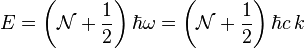E=\left( \mathcal N + \frac 12\right)\hbar\omega = \left(\mathcal N + \frac 12 \right) \hbar c\, k

$\mathcal N$ corresponds to the "number of photons" associated with a given normal mode. At a sufficiently low temperature, we may take $\mathcal N = 0$ as a reasonable approximation and focus entirely on the ground state energy. For simplicity, we shall also adopt units where $\hbar = c =1$ . Hence, energy, E, wavenumber, k = 2π/λ, and angular frequency, ω, all have the same units. Taking two polarizations for each normal mode of standing waves in a box with spatial dimensions $a\times L\times L$ , the three-dimensional sum over all possible wavenumbers yields,

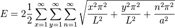
E = 2\frac{1}{2} \sum_{x=1}^{\infty}\sum_{y=1}^{\infty}\sum_{n=1}^{\infty}\sqrt{\frac {x^2\pi^2}{L^2}+\frac {y^2\pi^2}{L^2}+\frac {n^2\pi^2}{a^2}}

To keep the mathematics simple, we consider the artificial one-dimensional "box" of length $a$ , and instead, consider this sum:

\frac{aE}{\pi} \equiv S = \sum_{n=1}^{\infty}n = 1 + 2 + 3 + 4 + ...

Exponential regularization

Our first task is to regularize this divergent series by replacing it with something more manageable. Each integer represents a successively larger wavenumber. It is reasonable to assume that this summation ceases to be valid above some threshold energy. For example, metal ceases to be a good conductor at high frequency due to the skin effect. In cosmology, the energy/mass equivalence seems to imply an infinite source of gravity. Exponential regularization is one of many ways to model this cuttoff above some threshold frequency. Loosely speaking, Σn=Σne^−α in the limit that α vanishes, but the regularized sum in not an analytic function of α at α = 0.

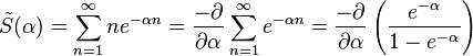
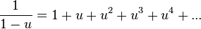
\tilde S(\alpha) = \sum_{n=1}^{\infty}ne^{-\alpha n} =\frac{-\partial}{\partial\alpha}\sum_{n=1}^{\infty}e^{-\alpha n} =\frac{-\partial}{\partial\alpha}\left(\frac{e^{-\alpha }}{1-e^{-\alpha }}\right)

where the last step defined u=e^−α and used the well-known result for $|u|<1\,$ ,

\frac{1}{1-u}=1+u+u^2+u^3+u^4+...

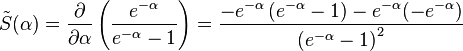
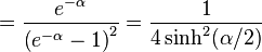
Using the quotient rule to evaluate the derivative, we obtain^[4]:

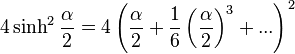
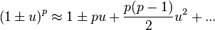
\tilde S(\alpha) = \frac{\partial}{\partial\alpha}\left(\frac{e^{-\alpha }}{e^{-\alpha} -1}\right)= \frac { - e^{-\alpha} \left(e^{-\alpha}-1\right) - e^{-\alpha}(-e^{-\alpha}) } { \left( e^{-\alpha} - 1 \right)^2 }

=\frac { e^{-\alpha }} { \left( e^{-\alpha } - 1 \right)^2 } =\frac{1}{4\sinh^2(\alpha/2)}

Consider the following Taylor expansion around α = 0:

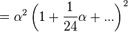
4\sinh^2 \frac\alpha 2 = 4\left( \frac\alpha 2 + \frac 1 6 \left(\frac\alpha 2\right)^3 + ...\right)^2

= \alpha^2 \left( 1 + \frac {1} {24} \alpha + ...\right)^2

Use this approximation to take the square of the inverse:

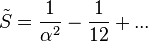
\left(1\pm u\right)^p\approx 1\pm pu + \frac{p(p-1)}{2}u^2 + ...

\tilde S = \frac{1}{\alpha^2}-\frac{1}{12} + ...

click to see higher order terms

Higher order terms can be shown to involve Bernoulli numbers ^[5]

\tilde S = \frac{1}{\alpha^2}-\frac{1}{12} + \frac{1}{240}\alpha^2 - \frac{1}{6048}\alpha^4 + \frac{1}{1278000}\alpha^6 +...

optional:using MATLAB to calculate the higher order terms

click to view

The code that follows Taylor expands the inverse of sinh(x/2) and then Taylor expands the inverse of the Taylor expansion. This proved simpler than sorting out w:L'Hôpital's_rule on a fraction in which both the numerator and denominator vanish in the limit of interest.

For a MATLAB investigation of another type of exponential regularization, see MATLAB/Divergent series investigations

% This MatLab code Taylor expands the S function.
clear all; clc; close all;%Start all codes with these 3 statements.
syms x  Establishes x as a symbol
f=@(x) x^2/(sinh(x/2))^2;
ftay=taylor(f(x),'Order',3);  %Supresses the fourth order term for printout
S = ftay/4/x^2;
fprintf('Keeping only the first two terms,\n 1+2+3+...= %s \n',char(S))
% Now do the high order terms
ftay=taylor(f(x), 'Order', 11);
S = ftay/4/x^2;  %prints out S to higher order
fprintf('Keeping many terms,\n 1+2+3+...= %s \n',char(S));
fprintf('Using the function pretty yields \n');
pretty(S)

Output:

     10        8       6      4    2
    x         x       x      x    x
  ------- - ------ + ---- - --- + -- - 1
  5322240   172800   6048   240   12
- --------------------------------------
                     2
                    x

Interpretation

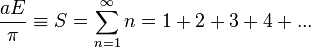
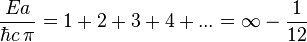
Loosely speaking, the wave energy, E, and length of our one dimensional box, a, are related by^[6],

\frac{Ea}{\hbar c\,\pi}=1+2+3+4+... = \infty - \frac{1}{12}

We shall soon see that the infinity is exactly cancelled out by the ground-state energy density that exists outside the two plates, in a region of space we shall call the "universe". Then we shall argue that regularization is not a mysterious mathematical trick, but a physically realistic model that represents the fact that metal is not a good conductor at sufficiently high frequency. Moreover, no harm was done by assuming exponential regulation, since any sufficiently smooth high-frequency cutoff yields the same result.

In order to assign a physical meaning to $\alpha$ , define a critical mode number $n_c$ associated with the high energy/frequency cutoff:

e^{-\alpha n}= e^{-n/n_c}

The contribution of each mode to total energy begins to fall by a factor of e at this wavenumber:

\kappa_c=\frac{n_c\pi}{a} \, ,

from which we conclude that $\alpha=\frac{\pi}{\kappa_c a}$ . The total energy in our one-dimensional box is:

E = \frac\pi a \left[\frac{1}{\alpha^2}-\frac{1}{12} \right]=\frac{a\kappa_c^2}{\pi}-\frac{\pi}{12a}

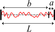
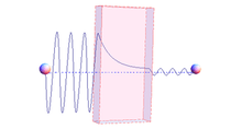
Casimir effect in one dimension. The parallel plates are separated by length, a, and the large segment of length b represents the rest of the "universe".

The Casimir force is caused by the change in total energy when the length, a, changes. Let our universe consist of a very large box of length, L, as shown in the figure. Ground state photon modes exist in two boxes, one of length, a, and the other of length b = L − a. The total energy is U = E_a+E_b

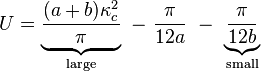
$U= \underbrace{ \frac{(a+b)\kappa_c^2}{\pi} } _{\mathrm{large}} \ - \ \frac{\pi}{12a} \ - \ \underbrace{\frac{\pi}{12b}} _{\mathrm{small}}$

The large term plays no role in calculating the force because it is constant (since a + b = L). The small term may be neglected because b >> a. Also, it should be noted that the force, F = −∂U/∂x is larger in this artificial one-dimensional model than it would be for actual parallel plates in three dimensions.

The Casimir effect holds for any sufficiently gentle regularization function

The choice of an exponential regularization function might seem arbitrary to some readers. Here we show that the same result is obtained for any sufficiently gentle regularization of the infinite series, 1+2+3+4+....

The trapezoidal rule is equivalent to a centered Riemann sum that either overestimates or underestimates the integral (depending on the sign of the second derivative).

The first step is to convince yourself that,

\int_{0}^{x_{N}} f(x)\,dx \approx h\left(\frac{f_{0}}{2} + f_1 +f_2+...+ f_{N-1} + \frac{f_{N}}{2} \right) + \frac{h^2}{12}\left(f'_0 - f'_N\right)

where we have subdivided the integral as a Riemann sum with intervals of length h.

click for plausibility argument

The aforementioned equation represents the first two terms of the Euler–Maclaurin formula, which is hard to prove:

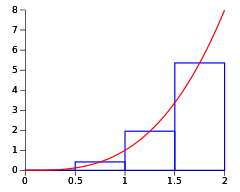
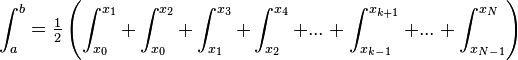
\int_{0}^{x_{N}} f(x)\,dx = h\left(\frac{f_{0}}{2} + f_1 +f_2+...+ f_{N-1} + \frac{f_{N}}{2} \right) + \frac{h^2}{12}\left(f'_0 - f'_N\right) - \frac{h^4}{720}\left(f'''_0 - f'''_N\right)+ ...

To justify the first two terms of the Euler–Maclaurin formula we shall derive the trapezoidal rule in a way that estimates a first-order correction term:

\int_a^b f(x)\,dx =h\left(\frac{f_{0}}{2} + f_1 +f_2...+f_{N-1} + \frac{f_{N}}{2}\right) + \left[\begin{matrix} \mathrm{correction} \\ \mathrm{term}\end{matrix} \right]

We accomplish this by breaking the integral into integrals over many small segments:

\int_a^b = \tfrac 1 2 \left( \int_{x_0}^{x_1} + \int_{x_0}^{x_2} + \int_{x_1}^{x_3} + \int_{x_2}^{x_4} + ... +\int_{x_{k-1}}^{x_{k+1}}+... +\int_{x_{N-1}}^{x_{N}} \right)

where we have adopted the notation:

\int_{x_{k-1}}^{x_{k+1}}f(x)\, dx \equiv \int_{x_{k-1}}^{x_{k+1}}

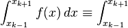
The factor of ½ arises from the fact that the integrals overlap so that each point in [a,b] is covered by two of the integrals. Except for the first and last integrals, each spans a length of 2h, or the range of three points along the real axis, 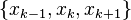$\{x_{k-1}, x_k, x_{k+1}\}$ .

Each integral is accomplished by by replacing the function by a parabola that is generated by the Taylor expansion,

\int_{x_{k-1}}^{ x_{k+1}}\left[ f_k + (x-x_k)f_k' + \frac 1 2 \right(x-x_k\left)^2f_k''\right]\,dx

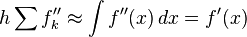
The first term yields the trapezoidal rule, the second term vanishes, and the third term can be summed to yield an expression that is related to the first derivatives at the two end-points via the approximation,

h\sum f_k'' \approx \int f''(x) \, dx = f'(x)

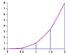
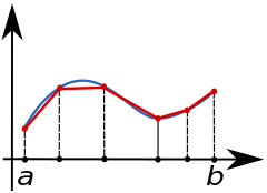
Where N is the number of points in the interval of integration, from $x_0$ to $x_N$ . Here, $f(x)=x$ initially, so that $f'_0=1$ . Then above some arbitrary large mode number, $f(x)$ must gradually level off and approach a situation where $f'(x)\to 0$ . In this equation, the integral (LHS^[7]) represents the continuum of states in the "universe" (outside the plates), and the sum (RHS) represents the spectrum of standing waves between the plates. The first, correction term, $\frac{h^2}{12}[f'_0 - f'_N]$ , represents the fact that in a regularized version of the theory, the sum must be slightly smaller than the integral. This line of reasoning suggests that it is the concave down nature of the regularization that explains why the plates are attracted.

Unsolved mystery? The question of why adopting the asymmetric boundary conditions^[8] causes the plates to attract must remain as an unsolved mystery.

Regularization is not an artificial "trick"

This is an eigenstate of a classical wave. At higher frequencies the leakage between the plates is greater, and this effect offers physical justification for regularization of the divergent series.

The quantum field theory used to develop this model is based on the classical wave equation. This classical wave equation can also be used to model finite resistivity of the wave equation, and can also be quantized, provided the wave equation is not dissipative. (Quantum theories are largely incompatible with friction or any other dissipative effect.) All that is necessary to achieve second quantization is to express the wave Hamiltonian in terms of eigenstates of the classical wave equation.

To better model the Casimir effect, one might assume that an inductive impedance dominates at high frequencies. It seems to me'^[9] that this would cause the low frequency eigenstates to be segregated by the plates, but cause the high frequency eigenstates to occupy both sides of the plate. This would gradually reduce the difference in energy density between the two spatial regions, causing a careful calculation to yield a regularized version of the infinite series 1+2+3+4+.... The previous section showed that the result does not depend on the nature of this regularization, provided the transition from confined (e.g. radio waves) to unconfined waves (e.g. X-rays) is sufficiently gradual.

It does not seem that exponential regularization of the series, 1+2+3+4+..., is an artificial trick. In fact, it informs us that the mechanism that causes the Casimir effect is that at sufficiently high frequencies, the ground-state electromagnetic energy levels are not restricted to the region between the plates. This creates a frequency range in which the waves begin to "leak" or "tunnel" between two locations (i.e. between the plates and outside them). Regularization informs us that if we know the high-frequency cut-off for confinement of standing waves by the plates, then we will know what frequencies are largely responsible for the Casimir effect. This transition regime consists of frequencies for which the penetration through the metal plates is considerable but not so large that the plates are essentially transparent.

This is one of four Wikiversity resources on divergent series

Other references

↑ the video had 2.5 million hits as of November 2014
↑ pun intended
↑ The only requirement is that the wave energy be proportional to the square of the wave amplitude integrated over all space. Also, for simplicity I assumed a scalar wave, although the same expression also holds for an EM wave.
↑ Bordag, Michael, Umar Mohideen, and Vladimir M. Mostepanenko. "New developments in the Casimir effect." Physics reports 353.1 (2001): 1-205 (see Equation 2.12 on page 12) http://arxiv.org/abs/quant-ph/0106045 and http://cecelia.physics.indiana.edu/journal/casimir_review.pdf See the same equation as Eq. 2.14 on page 19 of http://books.google.com/books?id=CqE1f_s5PgYC&pg=PA33#v=onepage&q&f=false
↑ http://mathworld.wolfram.com/BernoulliNumber.html
↑ Here we have reinserted the factor ħc convert the energy to conventional units.
↑ Left-hand side
↑ It seems to me that regularization always a produces concave down summation of confined normal modes. But see: Boyer, Timothy H. "Casimir forces and boundary conditions in one dimension: Attraction, repulsion, Planck spectrum, and entropy." American Journal of Physics 71.10 (2003): 990-998. http://arxiv.org/pdf/quant-ph/0211109v1.pdf
↑ I can't find the Wikiversity template that requests verification of an unsourced claim.

This article is issued from Wikiversity - version of the Friday, March 25, 2016. The text is available under the Creative Commons Attribution/Share Alike but additional terms may apply for the media files.