Quantum harmonic oscillator
The quantum harmonic oscillator is the quantum mechanical analogue of the classical harmonic oscillator. It is one of the most important model systems in quantum mechanics.
Hamiltonian
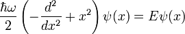
The Hamiltonian for the system is the following:
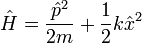
This Hamiltonian is a one dimensional Hamiltonian. Here is what each of the parts of the Hamiltonian mean:
- m is the mass of the particle
- The first term,
 is the usual kinetic energy term.
 - The second term,
 is the potential.
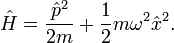
The potential term is very frequently written as 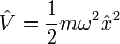 . This is because the spring constant k is related to the oscillator frequency via the relationship
  . When this is done, the Hamiltonian reads
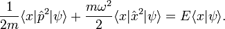
Time independent Schrödinger equation
The time independent Schrödinger equation is

and if we project onto the position basis, we get

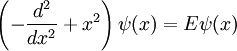
Substituting our Hamiltonian into the equation, we get
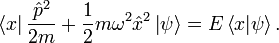
The constants can be pulled out in front of the bra  so the Schrödinger equation now reads
Now, consider the term  Recall that
  so
so 
For the other term  , recall that
 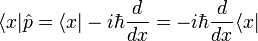 so that
  Putting all the pieces together, the Schrödinger equation reads
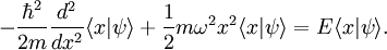
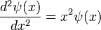
Since we are working in the position basis, we have  so we finally get
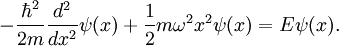
which is a differential equation which can be solved for  . This is of course, the wavefunction of the system in the position basis.
Solutions to the quantum harmonic oscillator
There are different approaches to solving the quantum harmonic oscillator. One of them, involves directly solving the differential equation which was obtained in the previous section. We will do this first. Afterwards, we will solve this same system with the "operator factorization method" as a way to motivate the introduction of boson operators into our quantum mechanical theory.
First, let's define a characteristic length for the quantum harmonic oscillator. We can do this heuristically by looking at the units involved in our expression.
-
 has units of
-
 has units of
-
 has units of
Hence, the quantity  has the units of length. We will call this length the "characteristic length". If we substitute into the differential equation
  we will get
Note also, that the units of  are also energy units. We can define
  as the characteristic energy of the system. (In fact, later, we will find that this energy happens to be the ground state zero point energy of the quantum harmonic oscillator.) So, putting
  we get
To solve this equation, first consider a simpler equation which describes the behaviour of the original wavefunction in some asymptotic limit. In the regime where the energy is very low,  , the wavefunction should then satisfy the differential equation
The form of this equation suggests that 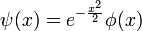 . Substituting
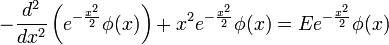

or

This differential equation can be solved in many different ways. One approach is to take
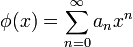
The derivatives are (note carefully the summation limits)
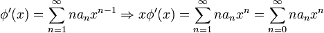
and similarily
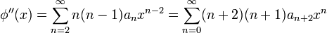
Substituting all of these terms into the above yields
![\sum_{n=0}^\infty x^n \left [ (n+2) (n+1) a_{n+2} - 2 n a_n + (E - 1) a_n \right ] = 0](../I/m/0135200ca8683a34cd664e5c13e344dc.png)
and vanishes term by term provided that
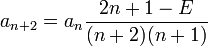
The most straightforward way to enforce these relationships is to set the numerator to zero. This leads to
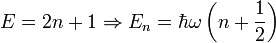
It's a very interesting result since the energy is now constrained to take on certain discrete values.
Feedback
This is still work in progress. Your feedback is appreciated! You're invited to leave comments on the talk page.