Physics/Essays/Fedosin/Quantum Inductance

< Physics < Essays < Fedosin

Quantum Inductance is the physical value that can be obtained from the density of states (DOS) approach, first introduced by Serge Luryi (1988) ^[1] to describe the 2D-electronic systems in silicon surfaces and AsGa junctions. This inductance is defined through standard density of states in the solids. Quantum inductance can be used in the w:Quantum Hall effect (integer and fractional) investigations as an approach which uses Quantum LC circuit.

Theory

Classical flat inductance

For the standard classical series $R_dL_dC_d \$ circuit the planar inductance can be defined as:

L_d = \frac{\mu_0 \mu_r S_{xz}N^2}{l_y},

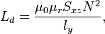
where $\mu_0 \$ is the vacuum permeability, $\mu_r \$ is the relative permeability, $S_{yz} = l_yl_z \$ is the MOSFET channel surface, $S_{xz} = l_xl_z \$ is the channel cross section, $l_x \$ is the channel depth, $l_y \$ is the channel length, $l_z \$ is the channel width, $N = \frac{l_y}{\lambda_y} \$ is the turn number of the planar induction coil, $\lambda_y \$ is the helix step of induction coil.

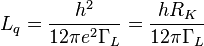
In the quantum limits, unknown parameter could be estimated by the following:

\lambda_y = \sqrt{\frac{\mu_0\mu_r S_{yz}l_x}{L_d}}

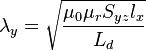where $\mu \to 1 \$ , $l_x \to \lambda_0 \$ , $L_d \to L \approx 7.407\cdot 10^{-2} \$ H and $S_{yz} \to S \approx 1.43\cdot 10^{-7} \$ m². Therefore we shall have the quantum value about Compton wavelength of electron 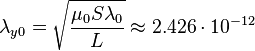$\lambda_0 \$ :

\lambda_{y0} = \sqrt{\frac{\mu_0 S \lambda_0 }{L}} \approx 2.426\cdot 10^{-12}

Quantum inductance in quantum tunneling

Josephson junction quantum inductance

Electromagnetic induction (Faraday) law is:

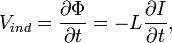
V_{ind} = \frac{\partial \Phi}{\partial t} = -L\frac{\partial I}{\partial t}, \

where $\Phi \$ is magnetic flux, $L \$ is the Josephson junction quantum inductance and $I \$ is the Josephson junction current.

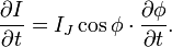
DC Josephson equation for current is:

I = I_J\cdot \sin \phi, \

where $I_J \$ is the Josephson scale for current, $\phi \$ is the phase difference between superconductors.

Current derivative on time variable will be:

\frac{\partial I}{\partial t} = I_J \cos \phi \cdot \frac{\partial \phi}{\partial t}. \

AC Josephson equation is:

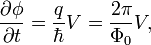
\frac{\partial \phi}{\partial t} = \frac{q}{\hbar}V = \frac{2\pi}{\Phi_0}V, \

where $\hbar \$ is the reduced Planck constant, $\Phi_0 = h/2e$ is the Josephson magnetic flux quantum, $q = 2e \$ and $e \$ is the elementary charge.

Combining equations for derivatives yields junction voltage:

V = \frac{\Phi_0}{2\pi I_J}\cdot \frac{1}{\cos \phi}\cdot \frac{\partial I}{\partial t} = L_J\cdot \frac{\partial I}{\partial t}, \

where

L_J = \frac{\Phi_0}{2\pi I_J}\cdot \frac{1}{\cos \phi} \

is the Deboret (1997) ^[2] quantum inductance.

DOS quantum inductance

In the general case 2D-density of states (DOS) in a solid can be defined by the following:

D_{2D} = \frac{m^*}{2\pi \hbar^2} \

where $m^* = \xi m_e \$ is current carriers effective mass in a solid, $m_e \$ is the electron mass, and $\xi \$ is a dimensionless parameter, which considers band structure of the solid. So, the quantum inductance can be defined as follows:

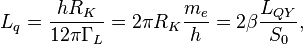
L_Q = \phi_0^2 \cdot D_{2D} \cdot S = \frac {h^2}{e^2} \cdot D_{2D} \cdot S = k \xi \cdot L_{Q0},

where $\phi_0 = h/e \$ is the magnetic flux quantum, $S = k S_0$ is the resonator surface area, $S_0 = \frac {\lambda^2_0}{2 \pi }$ is the elementary surface area, $k$ is the coefficient of area, $L_{Q0} = 2 \beta \cdot L_{QY} \$ is the elementary quantum inductance, and another ideal quantum inductance is:

L_{QY} = \mu_0 \lambda_0 = 3.04899 \cdot 10^{-18} \

where $\mu_0 \$ is the vacuum permeability, $\beta = \frac{1}{4\alpha} \$ is the magnetic coupling constant, $\alpha \$ is the fine structure constant and $\lambda_0 = \frac{h}{m_e c} \$ is the Compton wavelength of electron.

Quantum inductance in quantum Hall effect

The quantum inductance in the QHE mode will be:

L_{QA} = \frac{ \phi_0^2 \cdot D_{2D}}{n_B} \

where the carrier concentration per unit area in magnetic field $B \$ is:

n_B = \frac{eB}{h} .\

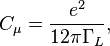
By analogy, the quantum capacitance in the QHE mode will be:

C_{QA} = \frac{ C_{QL}}{n_B} \

where

C_{QL} = e^2\cdot D_{2D} = \xi \cdot C_{q0},

is DOS definition of the quantum capacitance per unit area according to Luryi, ^[1] and $C_{q0} = 4\pi \alpha \cdot C_{qY} \$ is the elementary quantum capacitance per unit area at $\xi = 1 \$ , and another ideal quantum capacitance per unit area is: ^[3]

C_{qY} = \frac{\varepsilon_0}{\lambda_0} = 3.6492417 \

F/m²,

where $\varepsilon_0 \$ is the vacuum permittivity.

The standard wave impedance definition for the QHE LC circuit can be presented as:

\rho_Q = \sqrt{\frac{L_{QA}}{C_{QA}}} = \sqrt{\frac{\phi_0^2}{e^2}} = R_K \

where $R_K = \frac{h}{e^2} = 25.812813 k\Omega \$ is the von Klitzing constant for resistance.

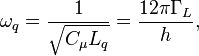
The standard resonant frequency definition for the QHE LC circuit can be presented as:

\omega_Q = \frac{1}{\sqrt{L_{QA}C_{QA}}} = \frac{\hbar \omega_c}{\phi_0e} = \frac{\omega_c}{2\pi}

where $\omega_c = \frac{eB}{m^*} \$ is the standard cyclotron frequency in the magnetic field $B \$ .

Quantum inductance per unit of area in a quantum dot

The first quantum inductance, based on the density of states approach was introduced by Wang et al. (2007) ^[4]. These authors modernized Buttiker approach (1993) ^[5] considering quantum dot (QD, labeled by “I”), placed over the metallic electrode (ME, labeled by “II”), and quantum capacitance. The quantum dot has the injected charge and induced charge per unit of area:

Q_I = Q_I^{inj} + Q_I^{ind} \

where injection charge is:

Q_I^{inj} = e^2 D_I v_I \

and induced charge is:

Q_I^{ind} = -e^2D_I V_I \

Therefore the resulting charge will be

Q_I = e^2D_I (v_I - V_I) = C_0 (V_I - V_{II}) = C_{\mu} (v_I - v_{II}) \

Q_{II} = - Q_I = e^2D_{II} (V_{II} - v_{II}) \

where $D_I \$ and $D_{II} \$ are frequency dependent density of states for QD and ME, $v_I \$ and $v_{II} \$ are the external AC potentials applied to the QD and ME and $C_{\mu}\$ is a frequency dependent capacitance per unit of area connected with the potentials; $V_I \$ and $V_{II} \$ are the proper frequency dependent electric potentials due to QD and ME, and $C_0 \$ is a capacitance per unit of area connected with the potentials.

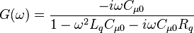
From the above we can obtain the following equation for the quantum capacitance per unit of area of the considered quantum system:

\frac{e^2}{C_{\mu}} = \frac{e^2}{C_0} + \frac{1}{D_I} + \frac{1}{D_{II} } \

The quantum density of states for QD as a function of frequency $\omega \$ can be expressed as:

D_I(\omega) = \frac{\Gamma_L}{2\pi \hbar \omega (\hbar \omega + i\Gamma_L)} \left [ \frac{1}{2} \ln \frac{\Delta^2}{\Delta_+\Delta_-} - i (\arctan \frac{\Delta E - \hbar\omega}{\Gamma_L/2} - \arctan {\frac{\Delta E + \hbar \omega}{\Gamma_L/2} }) \right ] ,

where $\Delta = \Delta E^2 + \Gamma_L^2/4 ,\$ and $\Delta_{\pm } = (\Delta E \pm \hbar \omega)^2 + \Gamma_L/4, \$ and $\Delta E = E_F - E_0 .\$

For the quantum capacitor at low frequencies, there exists a charge relaxation resistance: $R_q = \frac{h}{2e^2 \ }$ , for a single channel plate. Therefore, the considered system has the charge build-up time per unit of area due to the RC-time:

$\tau_{RC} = R_qC_{\mu} \$ .

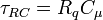However, the complexity of the density of states quantum capacitance produces another dwell time parameter $\tau_d \$ per unit of area, due to the quantum inductance. Actually, the general expression for quantum capacitance per unit of area can be expanded into a Taylor series to second order in frequency:

C_{\mu}(\omega) = C_{\mu 0} + i\omega C_{\mu 0}^2\frac{h}{2e^2} - \omega^2C_{\mu 0}^3\frac{h^2}{4e^4} + \omega^2C_{\mu 0}^2\frac{h^2}{12\pi \Gamma_Le^2} \

where $C_{\mu}(\omega =0) =C_{\mu}(0) = C_{\mu 0} \$ on the right hand side is the static electrochemical capacitance.

For a classical RLC circuit with capacitance $C_{\mu 0} \$ , resistance $R_q \$ and inductance $L_q \$ , the dynamic conductance is

G(\omega) = \frac{-i\omega C_{\mu 0}}{1 - \omega^2L_qC_{\mu 0}-i\omega C_{\mu 0}R_q} \

Expanding this expression in power series of $\omega \$ , we obtain

G(\omega) = -i\omega C_{\mu 0} + \omega^2C_{\mu 0}^2R_q + i\omega^3C_{\mu 0}^3R_q^2 - i\omega^3 C^2_{\mu 0}L_q \

Since a capacitor conductance 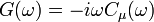$G(\omega) = -i\omega C_{\mu}(\omega) \$ , we obtain the following values for quantum resistance and inductance per unit of area:

R_q = h/2e^2 = R_K/2 \

L_q = \frac{h^2}{12\pi e^2\Gamma_L} = \frac{h R_K}{12\pi \Gamma_L} \

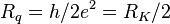where $R_K = \frac{h}{e^2} \$ is the von Klitzing constant.

Let us consider in more detail obtained values of reactive parameters of the system per unit of area:

C_{\mu} = \frac{e^2}{12 \pi \Gamma_L} ,\

L_q = \frac{h R_K}{12\pi \Gamma_L}= 2\pi R_ K\frac{m_e}{h} = 2 \beta \frac{L_{QY}}{S_0 } ,\

\tau_d = \frac{4\hbar}{\Gamma_L}, \

\omega_q = \frac{1}{ \sqrt{C_{\mu} L_q}} = \frac{12 \pi \Gamma_L}{h} ,\

\rho_q = \sqrt{\frac{L_q}{C_{\mu}}} = R_K , \

where line width function:

\Gamma_L = \frac{h^2}{24\pi^2m_e} = \frac{1}{12\pi}\frac{1}{D_{2D}} .\

So, we have the first definition of quantum inductance for the DOS.

Experiments

Quantum inductance in silicon MOSFETs

Semi-classical serial RLC circuit

In the general case the characteristic impedance of RLC circuit can be defined as:

Z_d = \sqrt{R_d + (\frac{1}{\omega C_d} - \omega L_d)^2} \

The resonant parameters of the RLC circuit (without dissipation, when $R_d =0\$ and $Z_d =0\$ ) will be:

\omega_d = \frac{1}{\sqrt{L_dC_d}} \

\rho_d = \sqrt{\frac{L_d}{C_d}} \

Semi-classical inductance and capacitance could be defined through the quantum values by the following: $L_d = L_0 + \Delta L \$ and $C_d = C_0 + \Delta C \$ .

So, the resulting value of quantum resonant impedance will be: $\rho_0 = \sqrt{\frac{L_0}{C_0}} = \sqrt{\frac{\mu_0}{\varepsilon_0}} \$ (impedance of free space).

Let us consider in more detail the semi-classical wave impedance in the form:

\rho_d = \sqrt{\frac{L_d}{C_d}} = \sqrt{\frac{L_0 + \Delta_L}{C_0 + \Delta_C}} \

Expanding this expression in power series of $\Delta_C \$ and $\Delta_L \$ , we shall obtain for the first order:

\rho_d = \rho_0[1 + \frac{1}{2}(\frac{\Delta_L}{L_0} - \frac{\Delta_C}{C_0})] \

Considering that $\Delta_L = L_d - L_0 \$ and $\Delta_C = C_d - C_0 \$ , the semi-classical wave impedance can be rewritten as:

\rho_d = \rho_0[1 + \frac{1}{2}(\frac{L_d}{L_0} - \frac{C_d}{C_0})] \

Experimental results

The first semi-classical resonant LC circuit was discovered by Yakymakha (1994) ^[3] during MOSFET spectroscopic investigation in the frequency band 100H – 20kH. Obtained value for the cycle resonance frequency (5088 rad/s), permits to make estimations for the quantum reactive MOSFETs parameters. Quantum capacitance was defined as:

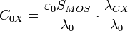
C_{0X} = \frac{\varepsilon_0S_{MOS}}{\lambda_0}\cdot \frac{\lambda_{CX}}{\lambda_0} \

where $S_{MOS} \$ is the MOSFET surface area and $\lambda_{CX} \$ is the flat quantum capacitance thickness.

Quantum inductance was defined as:

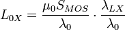L_{0X} = \frac{\mu_0S_{MOS}}{\lambda_0}\cdot \frac{\lambda_{LX}}{\lambda_0} \

where $\lambda_{LX} \$ is the flat quantum inductance thickness.

Experimental results prove that flat quantum inductance and capacitance thicknesses were about the Compton wavelength of electron:

\lambda_{CX} = \lambda_{LX} = \lambda_0 \

Quantum Hall Effect

The first attempts were made by Cage and Jeffery (1996) ^[6] to consider QHE devices as resonant LC circuit. These investigations were made due to the program of the AC-measuring resistor standards. However, the considered model used only classical approach to the reactive parameters of the Landau levels.

References

↑ 1.0 1.1 Serge Luryi (1988). "Quantum capacitance device". Appl.Phys.Lett. 52(6). Pdf
↑ Deboret M.H. (1997). "Quantum Fluctuations". Amsterdam, Netherlands: Elsevier. pp.351-386. Pdf
↑ 3.0 3.1 Yakymakha O.L., Kalnibolotskij Y.M. (1994). Very-low-frequency resonance of MOSFET amplifier parameters. Solid- State Electronics 37(10),1739-1751.
↑ Jian Wang, Baigeng Wang, and Hong Guo (2007). “Quantum inductance and negative electrochemical capacitance at finite frequency”. arXive:cond-mat/0701360v.Pdf
↑ M. Buttiker (1993). "Capacitance, admittance, and rectification properties of small conductors" J. Phys.: Condens. Matter 5, 9361. doi: 10.1088/0953-8984/5/50/017 Abstract
↑ M. E. Cage and A. Jeffery (1996).. “Intrinsic Capacitances and Inductances of Quantum Hall Effect Devices”. ‘’J. Res. Natl. Inst. Stand. Technol.’’ 101(6), 733 Pdf

External links

Jian Wang, Baigeng Wang, and Hong Guo (2007). "Quantum inductance and negative electrochemical capacitance at finite frequency in a two-plate quantum capacitor". Phys. Rev. B 75, 155336

This article is issued from Wikiversity - version of the Sunday, December 21, 2014. The text is available under the Creative Commons Attribution/Share Alike but additional terms may apply for the media files.