Physics Formulae/Waves Formulae
< Physics FormulaeLead Article: Tables of Physics Formulae
This article is a summary of the laws, principles, defining quantities, and useful formulae in the analysis of Waves.
General Fundamental Quantites
For transverse directions, the remaining cartesian unit vectors i and j can be used.
| Quantity (Common Name/s) | (Common) Symbol/s | SI Units | Dimension |
|---|---|---|---|
| Number of Wave Cycles |  | dimensionless | dimensionless |
| (Transverse) Displacement |  |
m | [L] |
| (Transverse) Displacement Amplitude |  |
m | [L] |
| (Transverse) Velocity Amplitude |  |
m s-1 | [L][T]-1 |
| (Transverse) Acceleration Amplitude |  |
m s-2 | [L][T]-2 |
| (Longnitudinal) Displacement |  |
m | [L] |
| Period |  | s | [T] |
| Wavelength |  |
m | [L] |
| Phase Angle |  |
rad | dimensionless |
General Derived Quantites
The most general definition of (instantaneous) frequency is:

For a monochromatic (one frequency) waveform the change reduces to the linear gradient:

but common pratice is to set N = 1 cycle, then setting t = T = time period for 1 cycle gives the more useful definition:
 |
| Quantity (Common Name/s) | (Common) Symbol/s | Defining Equation | SI Units | Dimension |
|---|---|---|---|---|
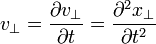
| (Transverse) Velocity |  |
 |
m s-1 | [L][T]-1 |
| (Transverse) Acceleration |  |
 |
m s-2 | [L][T]-2 |
| Path Length Difference |  |
 |
m | [L] |
| (Longnitudinal) Velocity |  |
 |
m s-1 | [L][T]-1 |
| Frequency |  |
|
Hz = s-1 | [T]-1 |
| Angular Frequency/ Pulsatance |  |
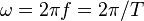 |
Hz = s-1 | [T]-1 |
| Time Delay, Time Lag/Lead |  |
 |
s | [T] |
| Scalar Wavenumber |  |
Two definitions are used:
In the formalism which follows, only the first definition is used. |
m-1 | [L]-1 |
| Vector Wavenumber |  |
Again two definitions are possible:
In the formalism which follows, only the first definition is used. |
m-1 | [L]-1 |
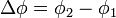
| Phase Differance |  |
 |
rad | dimensionless |
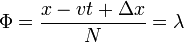
| Phase |  (No standard symbol, is used (No standard symbol, is used
only here for clarity of equivalances ) |
|
rad | dimensionless |
| Wave Energy | E | J | [M] [L]2 [T]-2 | |
| Wave Power | P |  |
W = J s-1 | [M] [L]2 [T]-3 |
| Wave Intensity | I |  |
W m-2 | [M] [T]-3 |
| Wave Intensity (per unit Solid Angle) | I | 
|
W m-2 sr-1 | [M] [T]-3 |


Phase
Phase in waves is the fraction of a wave cycle which has elapsed relative to an arbitrary point. Physically;
| wave popagation in +x direction
|
Phase angle can lag if: 
or lead if: |


Relation between quantities of space, time, and angle analogues used to describe the phase is summarized simply:
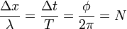 |
Standing Waves
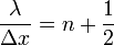
| Harmonic Number |  |
| Harmonic Series | 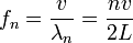 |
Propagating Waves
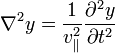
Wave Equation
Any wavefunction of the form
satisfies the hyperbolic PDE:
Principle of Superposition for Waves
General Mechanical Wave Results
| Average Wave Power | 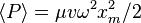 |
| Intensity | 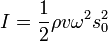 |
Sound Waves
Sound Intensity and Level
| Quantity (Common Name/s) | (Common) Symbol/s |
|---|---|
| Sound Level | 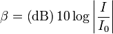 |
Sound Beats and Standing Waves
| pipe, two open ends | 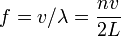 |
| Pipe, one open end | 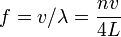 for n odd for n odd |
| Acoustic Beat Frequency | 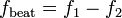 |
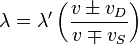
Sonic Doppler Effect
| Sonic Doppler Effect | 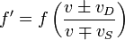
|
| Mach Cone Angle
(Supersonic Shockwave, Sonic boom) |
 |
Sound Wavefunctions
| Acoustic Pressure Amplitude | 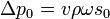 |
| Sound Displacement Function | 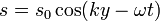 |
| Sound pressure-variation function | 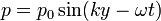 |
Superposition, Interferance/Diffraction
| Resonance |  |
| Phase and Interference | 
|

Phase Velocities in Various Media
The general equation for the phase velocity of any wave is (equivalent to the simple "speed-distance-time" relation, using wave quantities):
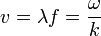 |
The general equation for the group velocity of any wave is:
 |
A common misconception occurs between phase velocity and group velocity (analogous to centres of mass and gravity). They happen to be equal in non-dispersive media.
In dispersive media the phase velocity is not necessarily the same as the group velocity. The phase velocity varies with frequency.
The phase velocity is the rate at which the phase of the wave propagates in space.
The group velocity is the rate at which the wave envelope, i.e. the changes in amplitude, propagates. The wave envelope is the profile of the wave amplitudes; all transverse displacements are bound by the envelope profile.
Intuitively the wave envelope is the "global profile" of the wave, which "contains" changing "local profiles inside the global profile". Each propagates at generally different speeds determined by the important function below called the Dispersion Relation , given in explicit form and implicit form respectivley.
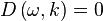 |
 |
The use of ω(k) for explicit form is standard, since the phase velocity ω/k and the group velocity dω/dk usually have convenient representations by this function.
For more specific media through which waves propagate, phase velocities are tabulated below. All cases are idealized, and the media are non-dispersive, so the group and phase velocity are equal.
| Taut String |  |
| Solid Rods |  |
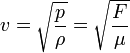
| Fluids |  |
| Gases | 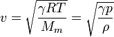 |
The generalization for these formulae is for any type of stress or pressure p, volume mass density ρ, tension force F, linear mass density μ for a given medium:
Pulsatances of Common Osscilators
Pulatances (angular frequencies) for simple osscilating systems, the linear and angular Simple Harmonic Oscillator (SHO) and Damped Harmonic Oscillator (DHO) are summarized in the table below. They are often useful shortcuts in calculations.
 = Spring constant (not wavenumber).
| Linear |  |
| Linear DHO | 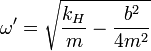 |
| Angular SHO |  |
| Low Amplitude Simple Pendulum |  |
| Low Amplitude Physical Pendulum |  |
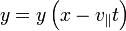
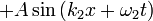
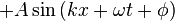
Sinusiodal Waves
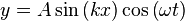
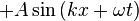
Equation of a Sinusiodal Wave is
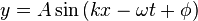
Recall that wave propagation is in  direction for
  .
.
Sinusiodal waves are important since any waveform can be created by applying the principle of superposition to sinusoidal waves of varying frequencies, amplitudes and phases. The physical concept is easily manipulated by application of Fourier Transforms.
Wave Energy
| Quantity (Common Name/s) | (Common) Symbol/s |
|---|---|
| potential harmonic energy |  |
| kinetic harmonic energy |  |
| total harmonic energy | 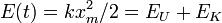 |
| damped mechanical energy | 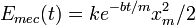 |
General Wavefunctions
Sinusiodal Solutions to the Wave Equation
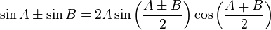
The following may be duduced by applying the principle of superposition to two sinusiodal waves, using trigonometric identities. Most often the angle addition and sum-to-product formulae are useful; in more advanced work complex numbers and Fourier series and transforms are often used.
| Wavefunction | Nomenclature | Superposition | Resultant |
| Standing Wave | 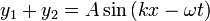
|
 | |
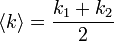
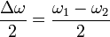
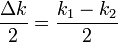
| Beats | 
|

|
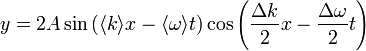 |
| Coherant Interferance |
|
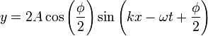 | |
Note: When adding two wavefunctions togther the following trigonometric identity proves very usefull:
Non-Solutions to the Wave Equation
| Exponentially Damped Waveform | 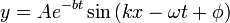 |
| Solitary Wave | |
Common Waveforms
| Triangular | |
| Square | |
| Saw-Tooth | |