Physics Formulae/Quantum Mechanics Formulae
< Physics FormulaeLead Article: Tables of Physics Formulae
This article is a summary of the laws, principles, defining quantities, and useful formulae in the analysis of Quantum Mechanics.
The nature of Quantum Mechanics is formulations in terms of probabilities, operators, matrices, in terms of energy, momentum, and wave related quantites. There is little or no treatment of properties encountered on macroscopic scales such as force.
Applied Quantities, Definitions
Many of the quantities below are simply energies and electric potential differances.
| Quantity (Common Name/s) | (Common) Symbol/s | Defining Equation | SI Unit | Dimension |
|---|---|---|---|---|
| Threshold Frequency | f0 |  |
Hz = s-1 | [T]-1 |
| Threshold Wavelength |  |
 |
m | [L] |
| Work Function |  |
 |
J | [M] [L]2 [T]-2 |
| Stopping Potential | V0 |  |
J | [M] [L]2 [T]-2 |
Wave Particle Duality
Massless Particles, Photons
| Planck–Einstein Equation | 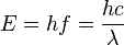 |
| Photon Momentum | 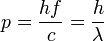 |
Massive Particles
| De Broglie Wavelength |  |
| Heisenberg's Uncertainty
Principle |

|

Typical effects which can only explained by Quantum Theory, and in part brought rise to Quantum Mechanics itself, are the following.
| Photoelectric Effect:
Photons greater than threshold frequency incident on a metal surface causes (photo)electrons to be emmited from surface. |
 |
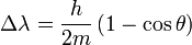
| Compton Effect
Change in wavelength of photons from an X-Ray source depends only on scattering angle. |
 |
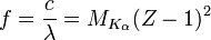
| Moseley's Law
Frequency of most intense X-Ray Spectrum (K-α) line for an element, Atomic Number Z. |
|
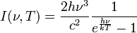
| Planck's Radiation Law
I is spectral radiance (W m-2 sr-1 Hz-1 for frequency or W m-3 sr-1 for wavelength), not simply intensity (W m-2). |
|
 Hz
Hz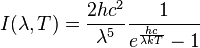
The Assumptions of Quantum Mechanics
| 1: State of a system | A system is completely specified at any one time by a Hilbert space vector. |
| 2: Observables of a system | A measurable quantity corresponds to an operator with eigenvectors spanning the space. |
| 3: Observation of a system | Measuring a system applies the observable's operator to the system and the system collapses into the observed eigenvector. |
| 4: Probabilistic result of measurement | The probability of observing an eigenvector is derived from the square of its wavefunction. |
| 5: Time evolution of a system | The way the wavefunction evolves over time is determined by Shrodinger's equation. |
Quantum Numbers
Quantum numbers are occur in the description of quantum states. There is one related to quantized atomic energy levels, and three related to quantized angular momentum.
| Name | Symbol | Orbital Nomenclature | Values |
|---|---|---|---|
| Principal | n | shell |  |
| Azimuth
Angular Momentum |
l | subshell;
s orbital is listed as 0, p orbital as 1, d orbital as 2, f orbital as 3, etc for higher orbitals |
 |
| Magnetic
Projection of Angular Momentum |
ml | energy shift (orientation of
the subshell's shape) |
 |
| Spin
Projection of Spin Angular Momentum |
ms | spin of the electron:
-1/2 = counter-clockwise, +1/2 = clockwise |
 |
Quantum Wave-Function and Probability
Born Interpretation of the Particle Wavefunction
Wavefunctions are probability distributions describing the space-time behaviour of a particle, distributed through space-time like a wave. It is the wave-particle duality characteristics incorperated into a mathematical function. This interpretation was due to Max Born.
Quantum Probability
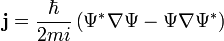
Probability current (or flux) is a concept; the flow of probability density.
The probability density is analogous to a fluid; the probability current is analogous to the fluid flow rate. In each case current is the product of density times velocity.
Usually the wave-function is dimensionless, but due to normalization integrals it may in general have dimensions of length to negative integer powers, since the integrals are with respect to space.
| Operator (Common Name/s) | (Common) Symbol/s | Defining Equation | SI Unit | Dimension |
|---|---|---|---|---|
| (Quantum) Wave-function | ψ, Ψ | 
|
m-n | [L]-n |
| Wavefunction, Probability Density Function | ρ | 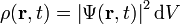 |
||
| Probability Amplitude | A, N | |||
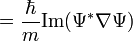
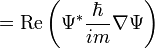
| Probability Current
Flow of Probability Density |
J, I | Non-Relativistic
|
||

Properties and Requirements
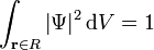
Normalization Integral
To be solved for probability amplitude.
R = Spatial Region Particle is definitley located in (including all space)
S = Boundary Surface of R.
 |
Law of Probability Conservation for Quantum Mechanics
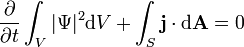 |
Quantum Operators
Observable quntities are calculated by operators acting on the wave-function. The term potential alone often refers to the potential operator and the potential term in Schrödinger's Equation, but this is a misconception; rather the implied quantity is potential energy .
It is not immediatley obvious what the opeators mean in their general form, so component definitions are included in the table. Often for one-dimensional considerations of problems the component forms are usefull, since they can be applied immediatley.
| Operator (Common Name/s) | Component Definitions | General Definition | SI Unit | Dimension |
|---|---|---|---|---|
| Position | 
|
 |
m | [L] |
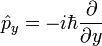
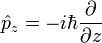
| Momentum | 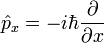
|
 |
J s m-1 = N s | [M] [L] [T]-1 |
| Potential Energy | 
|
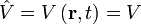 |
J | [M] [L]2 [T]-2 |
| Energy |  |
J | [M] [L]2 [T]-2 | |
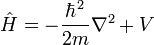
| Hamiltonian | 
|
J | [M] [L]2 [T]-2 | |
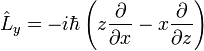
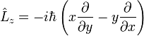
| Angular Momentum | 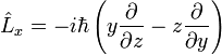
|
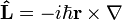 |
J s = N s m-1 | [M] [L]2 [T]-1 |
| Spin Angular Momentum | 
|
J s = N s m-1 | [M] [L]2 [T]-1 | |


Wavefunction Equations
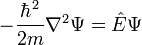
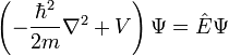
Schrödinger's Equation
General form proposed by Schrödinger:
 |
Commonly used corolaries are summarized below. A free particle corresponds to zero potential energy.
| 1D | 3D | |
|---|---|---|
| Free Particle (V=0) | 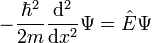 |
 |
| Time Independant | 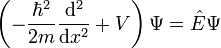 |
 |
| Time Dependant | 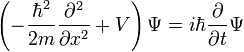 |
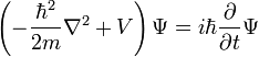 |
Dirac Equation
The form proposed by Dirac is
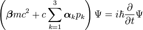 |
where  and
and  are Dirac Matrices satisfying:
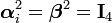
|


Klien-Gorden Equation
Schrödinger and De Broglie independantly proposed the relativistic form before Gorden and Klein, but Gorden and Klein included electromagnetic interactions into the equation, useful for charged spin-0 Bosons [1].
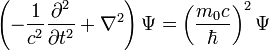 |
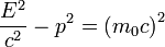
It can be obtained by inserting the quantum operators into the Momentum-Energy invariant of relativity:
Common Energies and Potential Energies
The following energies are used in conjunction with Schrödinger's equation (and other variants). In fact the equation cannot be used for calculations unless the energies defined for it.
The concept of potential energy is important in analyzing probability amplitudes, since this energy confines particles to localized regions of space; the only exception to this is the free particle subject to zero potential energy.
V0 = Constant Potential Energy
E0 = Constant Total Energy
| Potential Energy Type | Potential Energy V |
|---|---|
| Free Particle | 0 |
| One dimensional box | ![V = \begin{cases}
V_0 & x \in [a,b] \\
0 & x \notin [a,b]
\end{cases}
\,\!](../I/m/5c16de203df69ba5e898556d822d0d21.png) |
| Harmonic Osscilator |  |
| Electrostatic, Coulomb |  |
| Electric Dipole |  |
| Magnetic Dipole |  |
| Infinite Potential well | 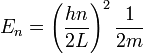
|
| Wavefunction of a Trapped
Particle, One Dimensional Box |
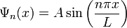
|
| Hydrogen atom, orbital energy | 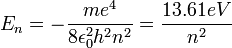
|

Quantum Numbers
Expressions for various quantum numbers are given below.
| spin projection quantum number | 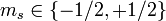 |
| Orbital Electron Magnetic Dipole Moment |  |
| Orbital Electron Magnetic Dipole Components |  |
| Orbital, Spin, Electron Magnetic Dipole Moment |  |
| Orbital Electron magnetic dipole moment |  |
| Orbital, Spin, Electron magnetic dipole moment Potential |  |
| Orbital, Electron Magnetic Dipole Moment Potential |  |
| Angular Momentum Components |  |
| Spin Angular Momentum Magnitude | 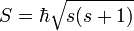 |
| Cutoff Wavelength |  |
| Density of States | 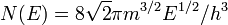 |
| Occupancy Probability |  |
Spherical Harmonics
The Hydrogen Atom
| Hydrogen Atom Spectrum,
Rydberg Equation |
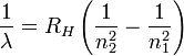 |
| Hydrogen Atom, radial probability density |  |
Referances
- ↑ Particle Physics, B.R. Martin and G. Shaw, Manchester Physics Series 3rd Edition, 2009, ISBN 978-0-470-03294-7