Physics Formulae/Conservation and Continuity Equations

Lead Article: Tables of Physics Formulae

This article is a summary of the laws, principles, defining quantities, and useful formulae in the analysis of Continuity and Conservation Equations.

To summarize essentails of physics, this section enumerates the classical conservation laws and continuity equations. All the following conservation laws carry through to modern physics, such as Quantum Mechanics, Relativity, Particle Physics and Quantum Relativity, though modifications to conserved quantities may be neccesary. Particle physics introduces new conservation laws, many in a different way using quantum numbers.

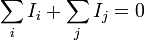
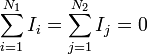
For any isolated system (i.e. independant of external agents/influences) the following laws apply to the whole system. Constituents of the system possesing these quantities may experiance changes, but the total amount of the quantity due to all constituents is constant.

Two equivalent ways of applying these in problems is by considering the quantities before and after an event, or considereing any two points in space and time, and equating the initial state of the sytem to the final, since the quantity is conserved.

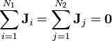
Corresponding to conserved quantities are currents, current densities, or other time derivatives. These quantites must be conserved also since the amount of a conserved quantity associated with a system is invariant in space and time.

Classical Conservation

Conserved Quantity	Constancy Equation	System Equation/s	Time Derivatives
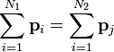
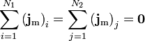
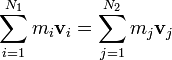
Mass	$\Delta m = 0 \,\!$	$M_{\mathrm{system}} = \sum_{i=1}^{N_1}m_i = \sum_{j=1}^{N_2}m_j \,\!$	Mass current conservation $\sum_{i=1}^{N_1} \left ( I_\mathrm{m} \right)_i = \sum_{j=1}^{N_2} \left ( I_\mathrm{m} \right)_j = 0\,\!$ $\sum_{i=1}^{N_1} \left ( \mathbf{j}_\mathrm{m} \right)_i = \sum_{j=1}^{N_2} \left ( \mathbf{j}_\mathrm{m} \right)_j = \mathbf{0} \,\!$
Linear Momentum	$\Delta \mathbf{p} = \mathbf{0} \,\!$	$\sum_{i=1}^{N_1} \mathbf{p}_{i} = \sum_{i=1}^{N_2} \mathbf{p}_{j} \,\!$ which can be written in equivalant ways, most useful forms are: $\sum_{i=1}^{N_1} m_i\mathbf{v}_i = \sum_{j=1}^{N_2} m_j\mathbf{v}_j$	Momentum current conservation $\sum_{i=1}^{N_1} \left ( I_\mathrm{p} \right)_i = \sum_{j=1}^{N_2} \left ( I_\mathrm{p} \right)_j = 0 \,\!$ Momentum current density conservation $\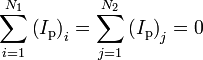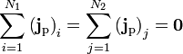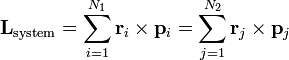sum_{i=1}^{N_1} \left ( \mathbf{j}_\mathrm{p} \right)_i = \sum_{j=1}^{N_2} \left ( \mathbf{j}_\mathrm{p} \right)_j = \mathbf{0} \,\!$
Total Angular Momentum	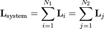$\Delta \mathbf{L}_\mathrm{total} = \mathbf{0} \,\!$	$\mathbf{L}_{\mathrm{system}} = \sum_{i=1}^{N_1}\mathbf{L}_i = \sum_{j=1}^{N_2}\mathbf{L}_j \,\!$ which can be written in equivalant ways, most useful forms are: $\mathbf{L}_{\mathrm{system}} = \sum_{i=1}^{N_1} \left ( \mathbf{I}_\mathrm{ab} \boldsymbol{\omega}_{\mathrm{b}} \right )_i = \sum_{j=1}^{N_2} \left ( \mathbf{I}_\mathrm{ab} \boldsymbol{\omega}_{\mathrm{b}} \right )_j \,\!$ $\mathbf{L}_{\mathrm{system}} = \sum_{i=1}^{N_1}\mathbf{r}_i \times \mathbf{p}_i = \sum_{j=1}^{N_2}\mathbf{r}_j\times \mathbf{p}_j \,\!$ $\mathbf{L}_{\mathrm{system}} = \sum_{i=1}^{N_1} m_i \left ( \mathbf{r}_i \times \mathbf{v}_i \right ) = \sum_{j=1}^{N_2}m_j \left ( \mathbf{r}_j\times \mathbf{v}_j \right )\,\!$	No analogue
Spin Angular Momentum	$\Delta \mathbf{L}_\mathrm{spin} = \mathbf{0} \,\!$	Same as above
Orbital Angular Momentum	$\Delta \mathbf{L}_\mathrm{orbital} = \mathbf{0} \,\!$	Same as above
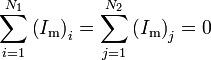
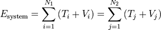
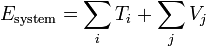
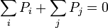
Energy	$\Delta E = 0 \,\!$	$E_\mathrm{system} = \sum_i T_i + \sum_j V_j \,\!$ or simply $E = T + V \,\!$ $E_\mathrm{system} = \sum_{i=1}^{N_1} \left ( T_i + V_i \right ) = \sum_{j=1}^{N_2} \left ( T_j + V_j \right ) \,\!$	Power conservation $\sum_i P_i + \sum_j P_j = 0\,\!$ Intensity conservation $\sum_i I_i + \sum_j I_j = 0\,\!$
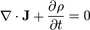
Charge	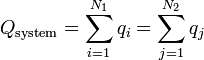$\Delta q = 0 \,\!$	$Q_{\mathrm{system}} = \sum_{i=1}^{N_1}q_i = \sum_{j=1}^{N_2}q_j \,\!$	Electric current conservation $\sum_{i=1}^{N_1} I_i = \sum_{j=1}^{N_2} I_j = 0 \,\!$ Electric current density conservation $\sum_{i=1}^{N_1} \mathbf{J}_i = \sum_{j=1}^{N_2} \mathbf{J}_j = \mathbf{0} \,\!$

Classical Continuity Equations

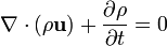
Continuity equations describe transport of conserved quantities though a local region of space. Note that these equations are not fundamental simply because of conservation; they can be derived.

Continuity Description	Nomenclature	General Equation	Simple Case
Hydrodynamics, Fluid Flow	$j_\mathrm{m} \,\!$ = Mass current current at the cross-section $\rho \,\!$ = Volume mass density $\mathbf{u} \,\!$ = velocity field of fluid $\mathbf{A} \,\!$ = cross-section	$\nabla \cdot (\rho \mathbf{u}) + {\partial \rho \over \partial t} = 0 \,\!$	$j_\mathrm{m} = \rho_1 \mathbf{A}_1 \cdot \mathbf{u}_1 = \rho_2 \mathbf{A}_2 \cdot \mathbf{u}_2 \,\!$
Electromagnetism, Charge	$I \,\!$ = Electric current at the cross-section $\mathbf{J} \,\!$ = Electric current density $\rho \,\!$ = Volume electric charge density $\mathbf{u} \,\!$ = velocity of charge carriers $\mathbf{A} \,\!$ = cross-section	$\nabla \cdot \mathbf{J} + {\partial \rho \over \partial t} = 0 \,\!$	$I = \rho_1 \mathbf{A}_1 \cdot \mathbf{u}_1 = \rho_2 \mathbf{A}_2 \cdot \mathbf{u}_2 \,\!$
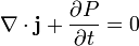
Quantum Mechnics, Probability	$\mathbf{j} \,\!$ = probablility current/flux $P = P(x,t) \,\!$ = probablility density function	$\nabla \cdot \mathbf{j} + \frac{\partial P}{\partial t} = 0 \,\!$

External Links

Conservation Laws

Continiuity Equations

This article is issued from Wikiversity - version of the Friday, July 17, 2015. The text is available under the Creative Commons Attribution/Share Alike but additional terms may apply for the media files.