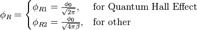
Physics/Essays/Fedosin/Quantum Electromagnetic Resonator
< Physics < Essays < FedosinA Quantum Electromagnetic Resonator (QER) – a closed topological object of the three dimensional space, in the general case – is a ‘’cavity’’ of arbitrary form, which has definite ‘’surface’’ and ‘’thickness’’. The QER has “infinite” phase shifted oscillations of electromagnetic field, due to its quantum properties.
History
It has happened, that such physical values as capacitance and inductance have no interest in the modern quantum electrodynamics. Furthermore, they are neglected even in classical electrodynamics, where electric and magnetic fields are dominated. The point is that, the last are not included in evident form in the Maxwell's equations, and so the resulting solutions includes fields only. Yes, sometimes these coefficients were obtained from the solutions of Maxwell equations, but it was very rarely.
It is known too, that s.c. “field approach” in electrodynamics that considered point charges leads to the “fool infinities”, as the interaction radius trends to zero. Furthermore, these “fool infinities” are presented in quantum electrodynamics too, where power methods are developed to compensate them.
Contrary to theoretical physics, applied physics has widely used reactive parameters, such as capacitance and inductance, firstly in electrotechnics and then in applied radiotechnics. Now reactive parameters are widely used in information technologies, which are based on the generation, transmission and radiation of electromagnetic waves of different frequencies.
The present day situation (without proper development of the theory of reactive parameters such as inductance, capacitance and electromagnetic resonator) prevents or slows developments in information technology and quantum computing. Note that, mechanical harmonic oscillator was considered in quantum mechanics in the early fourth decade of the twentieth century, when quantum theory was developed. However, quantum consideration of the  circuit was started only by Louisell (1973). [1]
Since then, there have been no practical examples of quantum capacitance and inductance, so this approach did not obtain proper consideration.
A theoretically correct introduction of quantum capacitance, based on the density of states, first was presented by Luryi (1988) [2] for QHE.
However, Luryi did not introduce quantum inductance, and this approach was not considered in quantum LC circuits and resonators. A year later, Yakymakha (1989) [3] considered an example of series and parallel quantum circuits (characteristic impedances) during QHE explanation (integer and fractional). However this work did not consider the Schrodinger equation for the quantum LC circuit.
For the first time, both quantum values, capacitance and inductance, were considered by Yakymakha (1994), [4] during spectroscopic investigations of MOSFETs at the very low frequencies (sound range). The flat quantum capacitances and inductances here had thicknesses about the Compton wave length of an electron, and its characteristic impedance – the wave impedance of free space.
And three year later, Devoret (1997) [5] presented a complete theory of the Quantum LC circuit (applied to the Josephson junction). Possible application of the quantum LC circuits and resonators in the quantum computation are considered by Devoret (2004). [6]
Classical electromagnetic resonator
In the general case, a classical electromagnetic resonator (CER) is a cavity resonator. It is a hollow closed conductor such as a metal box or a cavity within a metal block, containing electromagnetic waves reflecting back and forth between the cavity's walls. Therefore, a CER has infinite resonance frequencies, due to the three dimensions. For example, the rectangular CER has the following resonance frequencies:
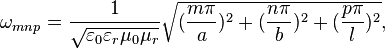
where  ;
;  are the width, thickness and length correspondingly,
 is the vacuum permittivity,
  is the relative permittivity,
 is the vacuum permeability,
  is the relative permeability.
Contrary to the classical LC circuit, both electric and magnetic fields are displaced in the same volume of CER.
These oscillating electromagnetic fields, in the classical case, are like standing waves, that form electromagnetic waves, that could be radiated to the external world.
Now CERs are widely used in the radio frequency range (centimetre and decimetre diapason). Furthermore, they are also used in quantum electronics, which deal with monochromic light waves.
Quantum general approach
Quantum LC circuit oscillator
In classical physics we have the following correspondence between mechanical and electrodynamical physical parameters:
Magnetic inductance and mechanical mass:
 ;
;
Electric capacitance and reciprocal elasticity:
 ;
;
Electric charge and coordinate displacement:
 .
.
The inductance momentum quantum operator in the electric charge space can be presented in the following form:

where  is the reduced Planck constant,
  is the complex-conjugate momentum operator.
The capacitance momentum quantum operator in magnetic charge space can be presented in the following form:

where  is the induced magnetic flux.
Considering that there is no free magnetic flux, but it could be imitated by electric current ( ):
):

we may introduce the third momentum quantum operator in the current form:

These quantum momentum operators define three Hamilton operators:
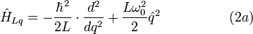
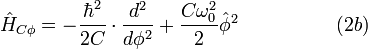
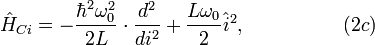
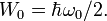
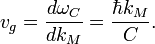
where  is the resonance frequency.
We consider the case without dissipation ( ).
).
The only difference of the charge spaces and current spaces here from the traditional 3D- coordinate space is that they are one dimensional (1D).
The Schrodinger equation for the quantum LC circuit may be defined in three forms:
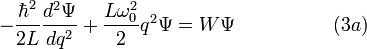
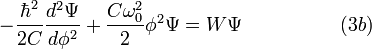
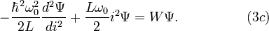
To solve these equations we introduce the following dimensionless variables:
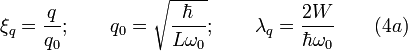
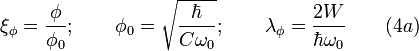
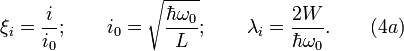
where  is scaling induced electric charge;
 is scaling induced magnetic flux and
 is scaling induced electric current.
Then the Schrodinger equation will take the form of the differential Chebyshev-Ermidt equation:
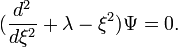
The eigenvalues of the Hamiltonian will be:
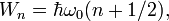
where at  we shall have zero oscillation:
In the general case the scaling charge and flux can be rewritten in the form:

where  is the fine structure constant.
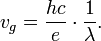
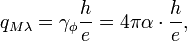
Furthermore, the scaling current and voltage will be here:

where  is the particle wavelength.
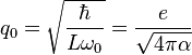
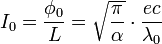
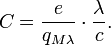
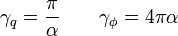
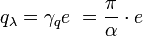
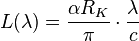
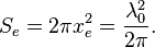
These scaling parameters were obtained by using the following quantum resonator parameters:

for characteristic impedance, and
for resonance frequency, and  is the von Klitzing constant. With this we have:

These three equations (3) form the base of a nonrelativistic quantum electrodynamics, which considers elementary particles from an intrinsic point of view. Standard quantum electrodynamics considers elementary particles from an external point of view.
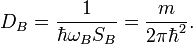
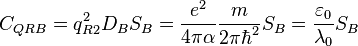
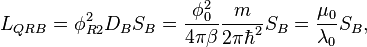
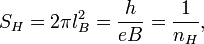
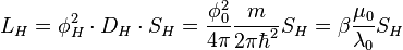
Resonator as quantum LC circuit
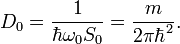
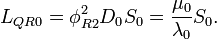
The Luryi density of states (DOS) approach defines quantum capacitance as:
and quantum inductance as:
where  is the resonator surface area,
 is two dimensional (2D) DOS,
 is the induced electric charge, and
 is the induced magnetic flux. Note that these charges should be defined afterward.
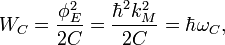
The energy stored on quantum capacitance:
The energy stored on quantum inductance:
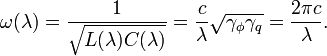
The resonator angular frequency is:
The energy conservation law for zero oscillation:
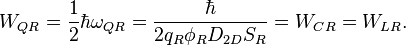
This equation can be rewritten as:

from which it is evident that induced charge and induced magnetic flux are connected to electric and magnetic fluxes in the resonator.
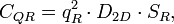
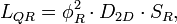
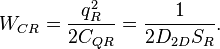
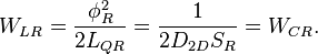
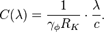
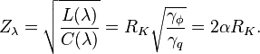
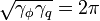
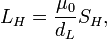
The characteristic resonator impedance is:

where  is the magnetic flux quantum,
 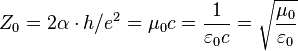 is the impedance of free space.
Considering the above equations, we have the following electric and magnetic sets of fluxes:
where 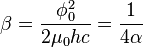 is the magnetic coupling constant.
These values are not the real charge and magnetic flux, but maximal quantities that maintain the energy balance between resonator oscillation energy and total energy on capacitance and inductance:

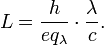
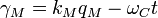
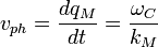
Since the capacitance oscillations are phase shifted ( ) with respect to inductance oscillations, we get:
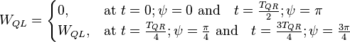
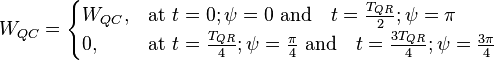
where  is the oscillation period.
De Broglie electromagnetic resonator
De Broglie matter wave [7] can be considered for the electric charge and magnetic flux. Actually, using the de Broglie approach in the form of Blohintzev [8] we can derive the following properties of charge quantum resonator (de Broglie charge bubble).
De Broglie electric charge
The electric charge in the de Broglie wave approach can be presented by the following wave function:
![\Psi(q_E,t) = A_E exp [i(\frac{\phi_Mq_E}{\hbar} - \frac{W_Lt}{\hbar})] = A_E exp [i(\gamma_E)] \](../I/m/f08e0510bb9bec33af21c566023610eb.png)
with


where  is electric charge "wave vector" and
 is electric charge "wave length".
The phase function
is electric charge "wave length".
The phase function
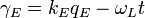
has differential

So, the phase current is:
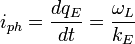
Considering wave energy in the form
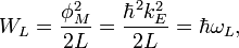
where  is de Broglie quantum inductance, and frequency

de Broglie "group current" will be:
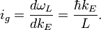
On the other hand, we have a limit for the group current:

Equating group currents, we may derive the de Broglie quantum inductance:
De Broglie magnetic flux
Magnetic flux in the de Broglie wave approach can be presented by the following wave function:
![\Psi(q_M,t) = A_M exp [i(\frac{\phi_E q_M}{\hbar} - \frac{W_Ct}{\hbar})] = A_M exp [i(\gamma_M)] \](../I/m/794a696cc2745c236a14c529670bcdcf.png)
with


where  is the space coordinate,
  is magnetic flux "wave vector" and
 is magnetic flux "wave length".
The phase function
is magnetic flux "wave length".
The phase function
has differential

The phase voltage will be:
Considering the wave energy in the form
where  is de Broglie quantum cdpacitance, and frequency

the de Broglie "group voltage" will be:
On the other hand we have the following limit for the group voltage:
Equating group voltages, we may derive de Broglie capacitance:
De Broglie LC circuit
Using separated electric and magnetic de Broglie charge approaches, we should consider the pilot wave approach to maintain electric and magnetic charges in a stable form. However, when we consider the composite de Broglie wave function in the following form:
![\Psi(q_M,t) = A_MA_E exp [i(\frac{\phi_Mq_E}{\hbar} - \frac{W_Lt}{\hbar})] exp [i(\frac{\phi_Eq_M}{\hbar} - \frac{W_Ct}{\hbar})] \](../I/m/98662ae16c274eaada2f2bccd38006c9.png)
with

then separated electric charge and magnetic flux produce a composite quantum resonator.
Considering that the de Broglie particle should be consistent with the quantum resonator, we determine the electric charge and magnetic flux induced in the LC circuit:


The reactive parameters in that case will be:
Characteristic impedance for the de Broglie charged particle resonator:
Resonance frequency for the de Broglie charged particle resonator:
Thus, we have the following algebraic system for unknown parameters:

The solution of this system is as follows:
Then, induced electric charge and magnetic flux may be rewritten as:
and reactive parameters are:

So, quantum oscillations of electric charge and magnetic flux make the charged de Broglie bubble stable in time.
Applications
Bohr atomic resonator
General information on Bohr atom. Bohr radius is:

where is the electric fine structure constant,
 is the Compton wavelength of electron.
Bohr surface scaling parameter for electron disc is:

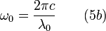
Bohr angular frequency is:

where is reduced Plank constant and  is electron mass.
Bohr density of states is:
Standard DOS quantum resonator approach yields the following values for the Bohr atom reactive quantum parameters:
where is the magnetic flux quantum, is the magnetic coupling constant.
Thus, s.c. "Bohr atom" could be considered as discoid quantum resonator which has radius  and thickness .
Electron resonator
Let suppose that the electron has its mass defined by the quantum oscillations, more precisely by the oscillations of the quantum LC circuit:

The oscillation length will be:

where  is the Compton wavelength of the electron.
Further, let us consider that the mass  is uniformly distributed on the electron surface:
Electron angular frequency is:
where  is the speed of light.
Then we can find out the density of states for this mass:
Standard DOS quantum resonator approach yields the following values for the electron reactive quantum parameters:
Thus, s.c. "free electron" could be considered as discoid quantum resonator which has radius  .
.
Photon resonator
As it is known, the photon momentum is defined as:

where is the speed of light,  is the energy of a photon.
So, the "effective (energy) photon mass" could be defined as:

Then the length scaling parameter of harmonic oscillator will be:
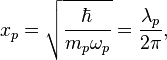
where  is the photon wavelength.
Photon surface scaling parameter is:
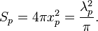
Photon angular frequency is:

Photon density of states is:
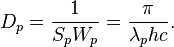
Standard DOS quantum resonator approach yields the following values for the photon reactive quantum parameters:
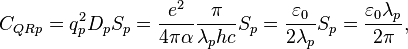
Thus, photon can be considered as quantum resonator which has radius  .
.
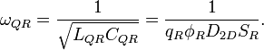
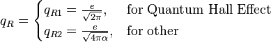
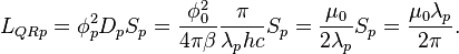
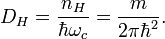
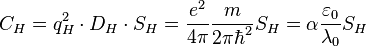
Quantum Hall resonator
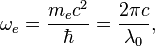
General information on the Hall resonator. Cyclotron frequency is:

where  is the elementary charge,
  is the magnetic field induction and is the electron effective mass in solid.
Magnetic length is:

Scaling area parameter is:
where  is the electron surface density.
Density of states is:
Density of states quantum capacitance is:
or in another form:
where  is the capacitance thickness.
Density of states quantum inductance is:
or in another form:
where 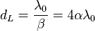 is the inductance thickness.
Thus, quantum Hall resonator has the cylindrical form with radius  and two different thickness:
  for capacitance and
  for inductance.
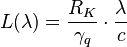
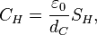
Flat atom resonator
A very low frequency resonance was discovered by Yakymakha (1994) [4] with mesoscopic parameters:
the angular frequency: 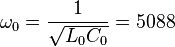 rad/s,
the surface scaling parameter: 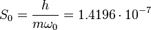 m2 ,
m2 ,
the quantum capacitance: 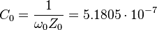 F, where
  is the impedance of free space,
the quantum inductance: 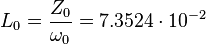 H.
H.
In the case of quantum resonator DOS will be:
Quantum resonator capacitance is:

where  .
.
Quantum resonator inductance is:
Note that, even in the mesoscopic case we have the reactive parameter thickness about Compton wave length of electron.
See also
- Physics/Essays/Fedosin/Quantum Hall composite resonator
- Quantum capacitance
- Quantum Inductance
- Quantum Gravitational Resonator
References
- ↑ Louisell W. H. (1973). “Quantum Statistical Properties of Radiation”. Wiley, New York.
- ↑ Serge Luryi (1988). "Quantum capacitance device". Appl.Phys.Lett. 52(6). Pdf
- ↑ Yakymakha O.L.(1989). High Temperature Quantum Galvanomagnetic Effects in the Two- Dimensional Inversion Layers of MOSFET's (In Russian). Kyiv: Vyscha Shkola. p.91. ISBN 5-11-002309-3. djvu.
- ↑ 4.0 4.1 Yakymakha O.L., Kalnibolotskij Y.M. (1994). "Very-low-frequency resonance of MOSFET amplifier parameters". Solid- State Electronics 37(10),1739-1751 Pdf.
- ↑ Deboret M.H. (1997). "Quantum Fluctuations". Amsterdam, Netherlands: Elsevier. pp.351-386. Pdf.
- ↑ Devoret M.H., Martinis J.M. (2004). "Implementing Qubits with Superconducting Integrated Circuits". Quantum Information Processing, v.3, N1. Pdf
- ↑ Louis de Broglie. The wave nature of the electron, Nobel Lecture, 12, 1929 PDF
- ↑ Блохинцев Д. И. Основы квантовой механики.- М.:ГосИздат, 1949.-588с.
Reference books
- Stratton J.A.(1941). Electromagnetic Theory. New York, London: McGraw-Hill.p.615. djvu
- Детлаф А.А., Яворский Б.М., Милковская Л.Б.(1977). Курс физики. Том 2. Электричество и магнетизм (4-е издание). М.: Высшая школа, "Reference Book on Electricity" djvu
- Гольдштейн Л.Д., Зернов Н.В. (1971). Электромагнитные поля. 2- издание. Москва: Советское Радио. 664с. "Electromagnetic Fields" djvu
Related papers
- Boris Ya. Zel’dovich. Impedance and parametric excitation of oscillators. UFN, 2008, v. 178, No 5 PDF