Normal distribution

A normal distribution can be described by four moments: mean, standard deviation, skewness and kurtosis. Statistical properties of normal distributions are important for parametric statistical tests which rely on assumptions of normality.

Probability density function

The probability density function of the standard normal distribution (with the standard deviation and area under the curve standardized to 1 and the mean and skewness standardized to 0) is given by $f(x)=\frac{e^{-x^2/2}}{\sqrt{2\pi}}$

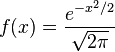
This function has no elementary antiderivative, and thus normal distribution problems are mainly limited to using numerical integration to find a probability. However, using multivariable calculus, the value of the Gaussian integral can be determined to be exactly 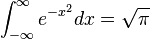$\int^{\infty}_{-\infty} e^{-x^2}dx = \sqrt{\pi}$ , and through the change of variables 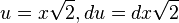$u=x\sqrt{2}, du=dx\sqrt{2}$ , we can be assured that the total area beneath the curve is 1, and thus it is normalized correctly.

A similar approach can be used to prove that its standard deviation is also 1. By the definition of the standard deviation, 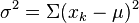$\sigma^2 = \Sigma{(x_k-\mu)^2}$ , so we form the Riemann sum 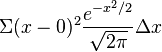$\Sigma (x-0)^2\frac{e^{-x^2/2}}{\sqrt{2\pi}} \Delta x$ . Taking the limit of the sum leads to the integral 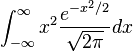$\int^{\infty}_{-\infty}x^2\frac{e^{-x^2/2}}{\sqrt{2\pi}} dx$ . Using integration by parts, we can determine that this is in fact equal to the area under the normal curve, and thus the standard deviation is 1. Using differentiation of the probability density function, we find that the inflection points of the normal distribution curve are each exactly one standard deviation away from the mean.

Any other normal distribution can be standardized through a change of variables (such as if the mean is not 0).

Histograms

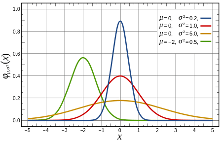Some normal distributions with various parameters.

Normal probability plots

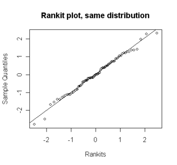A normality probability plot - data falling around this straight indicates the degree of departure from normality. For more information, see * Q-Q plot

Symbols

Population mean = μ (Mu)
Population variance = σ² = (Sigma squared)

Testing for normality

No single indicator of normality should be overly relied upon. Graphical, descriptive, and inferential can be used, each with strengths and limitations.

Graphical analysis

Histogram, with normal curve imposed
Normal Q-Q plot

Descriptive indicators of normality

A rule of thumb for assessing normality for the purposes of assumption testing for inferential statistical tests such as ANOVA is that if skewness and kurtosis are between -1 and +1 and there is a reasonable sample size (e.g., at least 20 per cell), then you are unlikely to run into issues related to violations of the assumption of normality.

The Skewness of a Normal Distribution is always 0.
The Kurtosis of a Normal Distribution is always 0.

Judging severity of skewness and kurtosis

Inferential tests of normality

Significance tests of (non-)normality become overly sensitive when the sample size is large. Thus, do not rely on significance tests of normality alone in making an assessment (e.g., for assumption-testing purposes):

Be aware that Shapiro-Wilks tends to be overly sensitive to minor departures from normality particular with large sample samples (e.g., > 200). This doesn't mean it should be discounted as an indicator, just that a sig. (p < .05) Shapiro-Wilks value does not necessarily indicate a notable deparature from normality. Check using other indicators.

In general, it is recommended that graphical indicators and descriptive indicators are used for inferential test assumption testing. Inferential tests may also be useful.

Dealing with non-normality

Transformations

Standardise data in SPSS

Non-parametric statistics

Non-parametric statistics

External links

Testing for normality using SPSS (Laerd Statistics]]

This article is issued from Wikiversity - version of the Monday, January 13, 2014. The text is available under the Creative Commons Attribution/Share Alike but additional terms may apply for the media files.