Nonlinear finite elements/Weak form of heat equation

Weak Form of the Heat Equation

Let us now derive the weak form of the model of heat conduction in equations (16). It is more convenient to use the form of the governing equation given in equation (10). The equation is

\rho~C_v~\frac{\partial T}{\partial t} - \boldsymbol{\nabla} \bullet [\boldsymbol{\kappa}\bullet\boldsymbol{\nabla T]} = s~.

Let $\mathcal{V}$ be the space of weighting functions (or test functions). Then any $w(\mathbf{x}) \in \mathcal{V}$ ( $\mathbf{x} \in \bar{\Omega}$ ) is continuously differentiable. The weighting functions also satisfy $w(\mathbf{x}) = 0$ on $\Gamma_T$ . Recall that we called a similar set of functions $\mathcal{X}$ in our discussion of the Poisson problem. We can write

\mathcal{V} = \{ w(\mathbf{x}) ~|~ \mathbf{x} \in \bar{\Omega},~ w(\mathbf{x}) \in \mathcal{H}^1(\Omega), ~\text{and}~ w(\mathbf{x}) = 0~\text{on}~ \Gamma_T\} ~.

Let $\mathcal{S}_t$ be the set of trial solutions. Then any trial function $T(\mathbf{x},t) \in \mathcal{S}_t$ has to satisfy the essential boundary conditions on $\Gamma_T$ . This is written as

\mathcal{S}_t = \{ T(\mathbf{x},t) ~|~ \mathbf{x} \in \bar{\Omega},~ t > 0, ~ T(\mathbf{x},t) \in \mathcal{H}^1(\Omega), ~\text{and}~ T(\mathbf{x},t) = \overline{T}(\mathbf{x},t) ~\text{on}~ \Gamma_T\} ~.

To get the weak form, we multiply the governing equation by the weighting function and integrate over the volume to get

\text{(28)} \qquad \int_{\Omega} \left(\rho~C_v~\frac{\partial T}{\partial t}\right)~w~dV - \int_{\Omega} \left[\boldsymbol{\nabla} \bullet (\boldsymbol{\kappa}\bullet\boldsymbol{\nabla T)}\right]~w~dV = \int_{\Omega} s~w~dV~.

The second term in the equation has second-order derivatives. We will convert these into first order derivatives using the divergence theorem and the identity

\boldsymbol{\nabla} \bullet (\varphi \mathbf{u}) = \varphi(\boldsymbol{\nabla} \bullet \mathbf{u}) + (\boldsymbol{\nabla} \varphi)\bullet\mathbf{u} ~.

From the identity we get

\text{(29)} \qquad w\left[\boldsymbol{\nabla} \bullet (\boldsymbol{\kappa}\bullet\boldsymbol{\nabla} T)\right] = \boldsymbol{\nabla} \bullet \left[w~(\boldsymbol{\kappa}\bullet\boldsymbol{\nabla} T)\right] - (\boldsymbol{\nabla} w)\bullet(\boldsymbol{\kappa}\bullet\boldsymbol{\nabla} T) ~.

Substitute (29) into the second term in (28) to get

\text{(30)} \qquad \int_{\Omega} \left[\boldsymbol{\nabla} \bullet (\boldsymbol{\kappa}\bullet\boldsymbol{\nabla} T)\right]~w~dV = \int_{\Omega} \boldsymbol{\nabla} \bullet \left[w~(\boldsymbol{\kappa}\bullet\boldsymbol{\nabla} T)\right]~dV - \int_{\Omega} (\boldsymbol{\nabla} w)\bullet(\boldsymbol{\kappa}\bullet\boldsymbol{\nabla} T)~dV ~.

Apply the divergence theorem to the first term on the right hand side of (30). You will get

\text{(31)} \qquad \int_{\Omega} \boldsymbol{\nabla} \bullet \left[w~(\boldsymbol{\kappa}\bullet\boldsymbol{\nabla} T)\right]~dV= \int_{\Gamma} \left[w~(\boldsymbol{\kappa}\bullet\boldsymbol{\nabla} T)\right]\bullet\mathbf{n}~dA

where $\mathbf{n}$ is the unit outward normal to the boundary $\Gamma$ .

Since $w(\mathbf{x}) = 0$ on $\Gamma_T$ , equation (31) becomes

\text{(32)} \qquad \int_{\Omega} \boldsymbol{\nabla} \bullet \left[w~(\boldsymbol{\kappa}\bullet\boldsymbol{\nabla} T)\right]~dV= \int_{\Gamma_q} \left[w~(\boldsymbol{\kappa}\bullet\boldsymbol{\nabla} T)\right]\bullet\mathbf{n}~dA~.

Substitute (31) into (30) and (30) back into (28). You will get

\text{(33)} \qquad \int_{\Omega} \left(\rho~C_v~\frac{\partial T}{\partial t}\right)~w~dV - \int_{\Gamma_q} \left[w~(\boldsymbol{\kappa}\bullet\boldsymbol{\nabla} T)\right]\bullet\mathbf{n}~dA + \int_{\Omega} (\boldsymbol{\nabla} w)\bullet(\boldsymbol{\kappa}\bullet\boldsymbol{\nabla} T)~dV= \int_{\Omega} s~w~dV~.

After rearrangement, we get the exact weak form of the heat equation

\text{(34)} \qquad { \int_{\Omega} \left(\rho~C_v~\frac{\partial T}{\partial t}\right)~w~dV + \int_{\Omega} (\boldsymbol{\nabla} w)\bullet(\boldsymbol{\kappa}\bullet\boldsymbol{\nabla} T)~dV= \int_{\Omega} s~w~dV + \int_{\Gamma_q} \left[w~(\boldsymbol{\kappa}\bullet\boldsymbol{\nabla} T)\right]\bullet\mathbf{n}~dA~. }

Recall that equation (15) gives us

-(\boldsymbol{\kappa}\bullet\boldsymbol{\nabla} T)\bullet\mathbf{n} = \overline{q} ~~\text{on}~~ \Gamma_q ~.

Therefore equation (34) can be written as

\text{(35)} \qquad { \int_{\Omega} \left(\rho~C_v~\frac{\partial T}{\partial t}\right)~w~dV + \int_{\Omega} (\boldsymbol{\nabla} w)\bullet(\boldsymbol{\kappa}\bullet\boldsymbol{\nabla} T)~dV= \int_{\Omega} s~w~dV - \int_{\Gamma_q} w~\overline{q}~dA~. }

In more compact notation

\text{(36)} \qquad { \langle w,~\rho~C_v~\dot{T\rangle} + a(w,~T) = \langle w,~s\rangle - \langle w,~\overline{q}\rangle_{\Gamma} ~. }

Following the same process for the initial condition, we get

\text{(37)} \qquad { \int_{\Omega} w~\left[\rho~C_v~T(0)\right]~dV = \int_{\Omega} w~\left[\rho~C_v~T_0\right]~dV ~. }

In compact notation,

{ \langle w,~\rho~C_v~T(0)\rangle = \langle w,~\rho~C_v~T_0\rangle ~. }

The variation initial boundary value problem for heat conduction can then be stated as follows.

 ${ \begin{align} & \mathsf{ Variational~ BVP ~for~ the ~Heat~ Equation}\\ & \\ \text{Find a function} & ~T(t) \in \mathcal{S}_t, t \in [0,\tau] ~\text{such that for all}~ w \in \mathcal{V}\\ & \\ & \int_{\Omega} \left(\rho~C_v~\frac{\partial T}{\partial t}\right)~w~dV + \int_{\Omega} (\boldsymbol{\nabla} w)\bullet(\boldsymbol{\kappa}\bullet\boldsymbol{\nabla} T)~dV= \int_{\Omega} s~w~dV - \int_{\Gamma_q} w~\overline{q}~dA \\ & \int_{\Omega} w~\rho~C_v~T(0)~dV = \int_{\Omega} w~\rho~C_v~T_0~dV ~. \end{align} }$

Well-Posedness of the Boundary Value Problem

Unless $\Omega$ has a simple geometry - square, spherical or cylindrical, it is very difficult to solve the BVP in closed form (using separation of variables, for instance). For some BVPs, it may not be possible at all to get a closed form solution. In fact, it may not even be obvious that a solution exists or is unique or that the solution depends continuously on the data.

A well-posed problem is one that satisfied the three conditions:

a solution exists.
the solution is unique.
the solution depends continuously on the data (that is, smallchanges in the data do not cause wild fluctuations in the solution).

BVPs can be used to get reliable results only when they are well-posed.

Let us look at an example. Recall the BVP for the Poisson equation.

 ${ \begin{align} & &\mathsf{ Poisson's~ equation}\\ & & \\ & \text{PDE:}~~~ &~~~- \nabla^2 T = f ~~\text{in}~~\Omega\quad\\ & \text{BCs:}~~~ &~~~ T = \overline{T}(\mathbf{x})~~\text{on}~~\Gamma_T ~~\text{and}~~ \frac{\partial T}{\partial n} = g(\mathbf{x})~~\text{on}~~\Gamma_q\quad\\ \end{align} }$

Assume that $\Gamma = \Gamma_q$ . That means that the heat flux is given on the entire boundary.

Suppose $T$ is a solution. Then $T+c$ is also a solution, where $c$ is a constant. To see why, compute the Laplacian of $T+c$ .

\nabla^2 (T+c) = \boldsymbol{\nabla} \bullet [\boldsymbol{\nabla (T+c)]} = \boldsymbol{\nabla} \bullet (\boldsymbol{\nabla T)} = \nabla^2 T~.

So the solution $T+c$ satisfies the PDE.

How about the boundary conditions?Plug in $T+c$ into the boundary condition to get

\frac{\partial (T+c)}{\partial n} = [\boldsymbol{\nabla} (T+c)]\bullet\mathbf{n} = (\boldsymbol{\nabla} T)\bullet\mathbf{n} = \frac{\partial T}{\partial n}

So the boundary conditions are also satisfied. That means that if $\Gamma_T = \varnothing$ , then the solution is not unique. We can add any constant temperature to the body and the solution will be consistent with the governing equations.

We can also check the conditions under which a solution will exist for this problem. Integrate the Poisson equation over $\Omega$ to get

\int_{\Omega} \nabla^2 T~dV = - \int_{\Omega} f~dV.

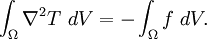
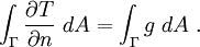
Apply the divergence theorem to the Laplacian. We get

\int_{\Omega} \nabla^2 T~dV = \int_{\Omega} \boldsymbol{\nabla} \bullet (\boldsymbol{\nabla T)}~dV = \int_{\Gamma} \mathbf{n}\bullet\boldsymbol{\nabla} T~dA \int_{\Gamma} \frac{\partial T}{\partial n}~dA.

From the boundary condition,

\int_{\Gamma} \frac{\partial T}{\partial n}~dA = \int_{\Gamma} g~dA~.

Therefore, we have

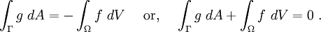
\int_{\Gamma} g~dA = - \int_{\Omega} f~dV~~~~\text{or,}~~~~ { \int_{\Gamma} g~dA + \int_{\Omega} f~dV = 0~.}

The boxed equation is called a compatibility condition and a solution does not exist unless this condition is satisfied.

In the context of the steady heat conduction problem, the compatibility condition says that the heat generated in the body must equal the heat flux. A similar (but more complicated) exercise can be used to show the existence and uniqueness of solutions for the full heat equation.

This article is issued from Wikiversity - version of the Tuesday, August 14, 2007. The text is available under the Creative Commons Attribution/Share Alike but additional terms may apply for the media files.