Nonlinear finite elements/Weak form of Poisson equation
< Nonlinear finite elementsThe Equivalent Variational Problem
So far, we have seen mathematical models in PDE form. That is not the only way of developing a model even though it is commonly used.
Many finite element models are based on an alternative form called the variational problem. The problem is formulated as one where the goal is to minimize a functional.
The variational form and the partial differential equation form are equivalent for the same problem. Each can be derived from the other.
Let us look at a simplified problem - the Poisson equation. Simplify it further by assuming that the temperature is prescribed to be zero on the entire boundary.
Functional
The first stage is to find a functional that applies to the problem.This is the most difficult part of the process. One way of finding the right functional is to try out a number of different forms and see if they correspond to known differential equations. This process is relatively easy for linear problems but not for nonlinear problems.
Recall that a functional converts a function ( ) to a real number.
For the Poisson equation, we can find a functional by thinking in terms of the membrane problem. In that problem, the total potential energy is stored energy of the membrane minus the work done by the force. The functional can be written in the form
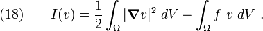
where  . The functional in equation (18)
represents the total potential energy of the membrane. The first term of
the functional represents the stored energy and the second term represents
the work done by the applied forces. For the membrane the solution is
the one that minimizes potential energy.
. The functional in equation (18)
represents the total potential energy of the membrane. The first term of
the functional represents the stored energy and the second term represents
the work done by the applied forces. For the membrane the solution is
the one that minimizes potential energy.
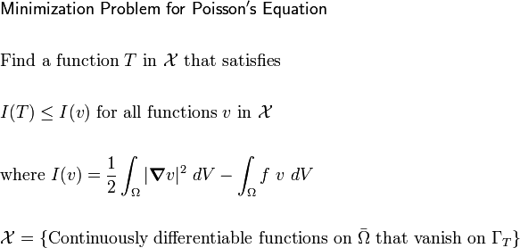
Since the same functional also works for the heat conduction problem (same PDE), we can minimize the functional to get at the temperature field that we seek.
Minimization problem
The Poisson equation for the heat conduction problem can then be written as

What are admissible functions? In brief, these are functions that satisfy the following requirements (in this particular case)
- They are continuously differentiable on
 where
where  .
. - They satisfy the boundary condition
 on
on  .
.
To summarize, the minimization problem is:
Finding a minimum
Let us take a simple function of one variable, say  . See
Figure 1(a). If a minimum exists, we can find it
by checking where the slope
. See
Figure 1(a). If a minimum exists, we can find it
by checking where the slope  .
.
A similar idea is used when we try to minimize a functional. See Figure 1(b).
For our problem, we have to find a minimizing function  from
the space of all admissible functions .
from
the space of all admissible functions .
The process of finding this minimizing function has the following steps:
- Assume that a minimizing function exists.
- Let this minimizing function be .
- Choose an arbitrary function
 .
. - Form a new function
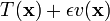 .
. - If we consider only the dependence of
 , we can treat the functional
  as a function only of , that is,
 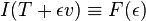 .
. - Now, the minimum is achieved when
 . Hence,
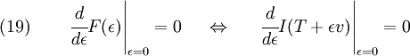
- Recall that the functional to be minimized is
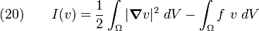
- Plug (20) into (19) and you will get
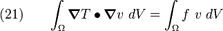
- (Show that this is true.)
- Equation (21) can be solved for and is called the variational boundary value problem.
The variational boundary value problem for the Poisson's equation form of the heat equation is
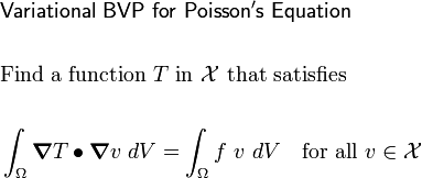
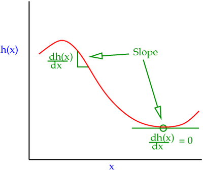 Figure 1(a). Minimizing a function. |
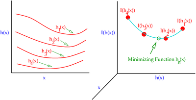 Figure 1(b). Minimizing a functional. |
Do I NEED to know the functional?
If the PDE form of the BVP is known, then we can derive the variational form directly from the PDE!
This process has the following steps:
- Start with the PDE BVP. Let's look at the Poisson equation for heat conduction as an example. The PDE is

- where
 .
.
- Choose an arbitrary function .
- Multiply (23) by
 and integrate over
  . We get
![\text{(24)} \qquad
- \int_{\Omega} (\nabla^2 T)~v~ dV = \int_{\Omega} f~v~ dV
~~~ \text{or,}~~~
- \int_{\Omega} [\boldsymbol{\nabla} \bullet (\boldsymbol{\nabla T})]~v~ dV = \int_{\Omega} f~v~ dV~.](../I/m/a17f53c753b8fa3407929992d29fd5e2.png)
- The left hand side of the equation has second derivatives. We want simplify things so that only first derivatives are involved. To do this, we use the identity

- where
 is a scalar valued function ( in our case), and
  is a vector valued function (like
  ). Apply this identity to the first term in equation (24). We get
 ![- \int_{\Omega} [\boldsymbol{\nabla} \bullet (v\boldsymbol{\nabla T)} - (\boldsymbol{\nabla} v)\bullet(\boldsymbol{\nabla} T)]
~ dV = \int_{\Omega} f~v~ dV~.](../I/m/aaf2ed3804292e7e1df7ef96a06adaff.png)
- Rearrange to get

- The first term is (25) still has second derivatives. Apply the Gauss divergence theorem
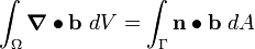
- where is a vector valued function and
 is the normal to the boundary
  . The first term of (25) becomes
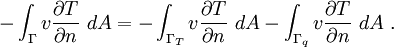
- The final form of (25) is called the Weak Form of the PDE and is written as

At this point, we can break the integral over the boundary into two parts -
an integral over and another over  , that is
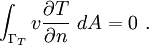
Recall that the function  has to meet the requirement that
on . Therefore,
has to meet the requirement that
on . Therefore,
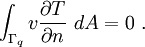
We also have the boundary condition that the boundary is insulated
( ) on . This implies that
Then, the weak form becomes
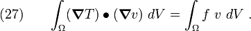
which is the same as the variational boundary value problem (21). We have arrived at the variational BVP without knowing the functional to be minimized!
Remarks
- Note that the variational BVP implicitly contains the flux boundary condition and we do not have to apply it separately when solving the BVP. This type of BC is called a natural boundary condition.
- The prescribed boundary condition is not satisfied by the variational BVP and has to be applied explicitly when solving the BVP. This type of BC is called an essential boundary condition.
You will often see the variational BVP (27)
written in the form
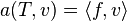
where
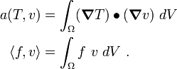
Here  is a linear functional
  acting on and
 is an example of a symmetric bilinear form.
A bilinear form is an operator that maps a pair of elements to the real
numbers, and which is linear in each of its slots. Let
is an example of a symmetric bilinear form.
A bilinear form is an operator that maps a pair of elements to the real
numbers, and which is linear in each of its slots. Let  and
and  be constants, and let
  , , and
  be functions. Then a bilinear
form has the properties that
be functions. Then a bilinear
form has the properties that
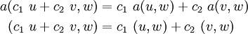
A symmetric bilinear form has the additional property that

(Show that equation (27) is actually a symmetric bilinear form.)