Introduction to Elasticity/Vectors
< Introduction to ElasticityVectors in Mechanics
Vector notation is ubiquitous in the modern literature on solid mechanics, fluid mechanics, biomechanics, nonlinear finite elements and a host of other subjects in mechanics. A student has to be familiar with the notation in order to be able to read the literature. In this section we introduce the notation that is used, common operations in vector algebra, and some ideas from vector calculus.
Vectors
A vector is an object that has certain properties. What are these properties? We usually say that these properties are:
- a vector has a magnitude (or length)
- a vector has a direction.
To make the definition of the vector object more precise we may also say that vectors are objects that satisfy the properties of a vector space.
The standard notation for a vector is lower case bold type (for example  ).
).
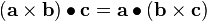
In Figure 1(a) you can see a vector  in red. This vector can be represented in component form with respect to the basis (
 ) as
) as
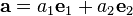
where  and
and  are orthonormal unit vectors. Recall that unit vectors are vectors of length 1. These vectors are also called basis vectors.
You could also represent the same vector in terms of another set of basis vectors ( ) as shown in Figure 1(b). In that case, the components of the vector are
  and we can write
Note that the basis vectors  and
and  do not necessarily have to be unit vectors. All we need is that they be linearly independent, that is, it should not be possible for us to represent one solely in terms of the others.
In three dimensions, using an orthonormal basis, we can write the vector as

where  is perpendicular to both and . This is the usual basis in which we express arbitrary vectors.
 Figure 1: A vector and its basis. |
Vector algebra
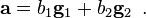
Some vector operations are shown in Figure 2.
 Figure 2: Vector operations. |
Addition and subtraction
If and  are vectors, then the sum
  is also a vector (see Figure 2(a)).
The two vectors can also be subtracted from one another to give another vector  .
.
Multiplication by a scalar
Multiplication of a vector by a scalar  has the effect of stretching or shrinking the vector (see Figure 2(b)).
You can form a unit vector  that is parallel to by dividing by the length of the vector
  . Thus,

Scalar product of two vectors
The scalar product or inner product or dot product of two vectors is defined as

where  is the angle between the two vectors (see Figure 2(b)).
If and are perpendicular to each other,  and
and  . Therefore,
  .
.
The dot product therefore has the geometric interpretation as the length of the projection of onto the unit vector  when the two vectors are placed so that they start from the same point.
The scalar product leads to a scalar quantity and can also be written in component form (with respect to a given basis) as
If the vector is  dimensional, the dot product is written as
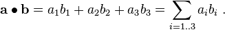
Using the Einstein summation convention, we can also write the scalar product as
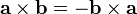
Also notice that the following also hold for the scalar product
 (commutative law).
 (distributive law).
Vector product of two vectors
The vector product (or cross product) of two vectors and is another vector  defined as

where is the angle between and , and  is a unit vector perpendicular to the plane containing and in the right-handed sense (see Figure 3 for a geometric interpretation)
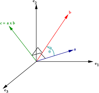 Figure 3: Vector product of two vectors. |
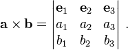
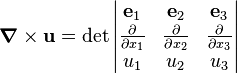
In terms of the orthonormal basis  , the cross product can be written in the form of a determinant
In index notation, the cross product can be written as
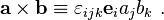
where  is the Levi-Civita symbol (also called the permutation symbol, alternating tensor).
Identities from vector algebra
Some useful vector identities are given below.
-
 .
. -
 .
. -
 .
. -
 .
. -
 .
. -
 .
. -
 .
.
Vector calculus
So far we have dealt with constant vectors. It also helps if the vectors are allowed to vary in space. Then we can define derivatives and integrals and deal with vector fields. Some basic ideas of vector calculus are discussed below.
Derivative of a vector valued function
Let  be a vector function that can be represented as

where  is a scalar.
Then the derivative of with respect to is

If and  are two vector functions, then from the chain rule we get
![\begin{align}
\cfrac{d({\mathbf{a}}\bullet{\mathbf{b}})}{dx} & =
{\mathbf{a}}\bullet{\cfrac{d\mathbf{b}}{dx}} + {\cfrac{d\mathbf{a}}{dx}}\bullet{\mathbf{b}} \\
\cfrac{d({\mathbf{a}}\times{\mathbf{b}})}{dx} & =
{\mathbf{a}}\times{\cfrac{d\mathbf{b}}{dx}} + {\cfrac{d\mathbf{a}}{dx}}\times{\mathbf{b}} \\
\cfrac{d[{\mathbf{a}}\bullet{({\mathbf{b}}\times{\mathbf{c}})}]}{dx} & =
{\cfrac{d\mathbf{a}}{dx}}\bullet{({\mathbf{b}}\times{\mathbf{c}})} +
{\mathbf{a}}\bullet{\left({\cfrac{d\mathbf{b}}{dx}}\times{\mathbf{c}}\right)} +
{\mathbf{a}}\bullet{\left({\mathbf{b}}\times{\cfrac{d\mathbf{c}}{dx}}\right)}
\end{align}](../I/m/038accc744b1de52cab75a4a2f1c5e91.png)
Scalar and vector fields
Let  be the position vector of any point in space. Suppose that
there is a scalar function (
be the position vector of any point in space. Suppose that
there is a scalar function ( ) that assigns a value to each point in space. Then

represents a scalar field. An example of a scalar field is the temperature. See Figure4(a).
 Figure 4: Scalar and vector fields. |
If there is a vector function () that assigns a vector to each point in space, then

represents a vector field. An example is the displacement field. See Figure 4(b).
Gradient of a scalar field
Let  be a scalar function. Assume that the partial derivatives of the function are continuous in some region of space. If the point has coordinates (
 ) with respect to the basis (
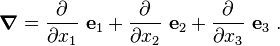
 ), the gradient of
  is defined as
In index notation,
The gradient is obviously a vector and has a direction. We can think of the gradient at a point being the vector perpendicular to the level contour at that point.
It is often useful to think of the symbol  as an operator of the form
Divergence of a vector field
If we form a scalar product of a vector field  with the operator, we get a scalar quantity called the
divergence of the vector field. Thus,
with the operator, we get a scalar quantity called the
divergence of the vector field. Thus,
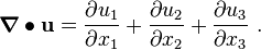
In index notation,
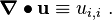
If  , then
  is called a divergence-free field.
The physical significance of the divergence of a vector field is the rate at which some density exits a given region of space. In the absence of the creation or destruction of matter, the density within a region of space can change only by having it flow into or out of the region.
Curl of a vector field
The curl of a vector field is a vector defined as
The physical significance of the curl of a vector field is the amount of rotation or angular momentum of the contents of a region of space.
Laplacian of a scalar or vector field
The Laplacian of a scalar field is a scalar defined as
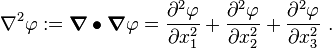
The Laplacian of a vector field is a vector defined as

Green-Gauss divergence theorem
Let be a continuous and differentiable vector field on a body  with boundary
  . The divergence theorem states that
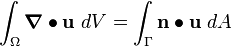
where  is the outward unit normal to the surface (see Figure 5).
In index notation,
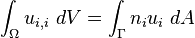
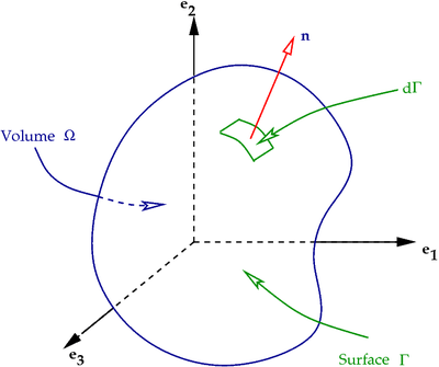 Figure 5: Volume for application of the divergence theorem. |
Identities in vector calculus
Some frequently used identities from vector calculus are listed below.
 .
. .
. .
. .
. .
.