Nonlinear finite elements/Updated Lagrangian approach
< Nonlinear finite elementsUpdated Lagrangian Approach
For the total Lagrangian approach, the discrete equations were formulated with respect to the reference configuration. For the updated Lagrangian approach, the discrete equations are formulated in the current configuration,which is assumed to be the new reference configuration.
The independent variables in the total Lagrangian approach were  and
and  . In the updated Lagrangian were
  and which are respect to the new reference configuration.
The dependent variable in the total Lagrangian approach was the the displacement  . In the updated Lagrangian approach, the dependent variables are the Cauchy stress
  and the velocity
  .
.
Updated Lagrangian Stress and Strain Measures
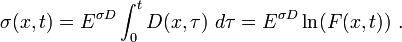
The stress measure is the Cauchy stress:
The strain measure is the rate of deformation (also called velocity strain):
Note that the derivative is a spatial derivative. It can be shown that
where  is the deformation gradient. So the integral of the rate of deformation in 1-D is similar to the logarithmic strain (also called natural strain).
Governing Equations in Updated Lagrangian Form
The Updated Lagrangian governing equations are:
Conservation of Mass

For the rod,
These are the same as those for the total Lagrangian approach.
Conservation of Momentum
In this case  may not be constant at along the length and
further simplification cannot be done. In short form,
may not be constant at along the length and
further simplification cannot be done. In short form,
Conservation of Energy
If we ignore heat flux and heat sources
If we include heat flux and heat sources
In short form:

Constitutive Equations
Total Form
For a linear elastic material:
The superscript  refers to the fact that this function
relates
refers to the fact that this function
relates  and
and  .
.
For small strains:
Rate Form
For a linear elastic material:
Initial and Boundary Conditions for Updated Lagrangian
For the updated Lagrangian approach, initial conditions are needed for the stress and the velocity. The initial displacement is assumed to be zero.
The initial conditions are:
![{
\begin{align}
\sigma(x,0) & = \sigma_0(x) & ~\text{for}~ & x \in [0, L] \\
v(x,0) & = v_0(x) & ~\text{for}~ & x \in [0, L]\\
u(x,0) & = 0 & ~\text{for}~ & x \in [0, L]
\end{align}
}](../I/m/2053c15783d261cbacad46aebdbc0807.png)
The essential boundary conditions are

The traction boundary conditions are

The unit normal to the boundary in the current configuration is
 . The tractions in the current configuration are related to those
in the reference configuration by
. The tractions in the current configuration are related to those
in the reference configuration by
The interior continuity or jump condition is

Weak Form for Updated Lagrangian
The momentum equation is
To get the weak form over an element, we multiply the equation by a
weighting function and integrate over the current length of the
element (from  to
to  ).
).
![\int_{x_a}^{x_b} w\left[(A~\sigma)_{,x} +
\rho~A~b - \rho~A~\cfrac{Dv}{Dt}\right]~dx = 0 ~.](../I/m/3e47b7a46375952767de10e0e5d558bc.png)
Integrate the first term by parts to get
![\int_{x_a}^{x_b} w (A~\sigma)_{,x}~dx = \left[w~A~\sigma\right]_{x_a}^{x_b} -
\int_{x_a}^{x_b} w_{,x}~(A~\sigma)~dx ~.](../I/m/d037d007c3e2124bab804d9eaa04e518.png)
Plug the above into the weak form and rearrange to get
![\int_{x_a}^{x_b} w_{,x}~(A~\sigma)~dx + \int_{x_a}^{x_b} w~\rho~A~\cfrac{Dv}{Dt}~dx =
\int_{x_a}^{x_b} w~\rho~A~b~dx + \left[w~A~\sigma\right]_{x_a}^{x_b} ~.](../I/m/2ed6313178069c6f9ab880cd472e8b80.png)
If we think of the weighting function  as a variation of
  that
satisfies the kinematic admissibility conditions, we get
the principle of virtual power:
that
satisfies the kinematic admissibility conditions, we get
the principle of virtual power:
![{
\int_{x_a}^{x_b} (\delta v)_{,x} (A~\sigma)~dx + \int_{x_a}^{x_b}\delta v~\rho~A~\cfrac{Dv}{Dt}~dx
=
\int_{x_a}^{x_b} \delta v~\rho~A~b~dx + \left[\delta v~A~\sigma\right]_{x_a}^{x_b} ~.
}](../I/m/3fc8327b60e3d71424c8c23b03a19c18.png)
Recall that

Therefore,
and
![\left[\delta v~A~\sigma\right]_{x_a}^{x_b} =
\left[\delta v~A~t_x\right]_{\Gamma_t} ~.](../I/m/4f708b88654c01419ac823eca8a7b663.png)
Hence we can alternatively write the weak form as
![{
\int_{x_a}^{x_b}\delta D~A~\sigma~dx + \int_{x_a}^{x_b}\delta v~\rho~A~\cfrac{Dv}{Dt}~dx =
\int_{x_a}^{x_b}\delta v~\rho~A~b~dx +\left[\delta v~A~t_x\right]_{\Gamma_t}~.
}](../I/m/8fc7fb8db1d6078156f8289995b8f0fc.png)
Comparing with the energy equation, we see that the first term above is
the internal virtual power. Using the substitutions  and
and
 , we can also write the weak form as
![{
\int_{\Omega}\delta D~\sigma~d\Omega +
\int_{\Omega}\delta v~\rho~\dot{v}~d\Omega =
\int_{\Omega}\delta v~\rho~b~d\Omega +\left[\delta v~A~t_x\right]_{\Gamma_t}~.
}](../I/m/8a3fa8d5765c90b08da6e78132150b41.png)
The weak form may also be written in terms of the virtual powers as

where,
![{
\begin{align}
\delta P_{\text{int}} & = \int_{x_a}^{x_b} (\delta v)_{,X}~(A~\sigma)~dx \\
\delta P_{\text{ext}} & = \int_{x_a}^{x_b} \delta v~\rho~A~b~dx +
\left[\delta v~A~t_X\right]_{\Gamma_t} \\
\delta P_{\text{kin}} & = \int_{x_a}^{x_b} \delta v~\rho~A~\dot{v}~dx
\end{align}
}](../I/m/f964931314670c9e18a5118c589d0b47.png)
Finite Element Discretization for Updated Lagrangian
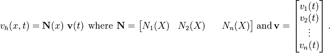
The trial velocity field is
In matrix form,
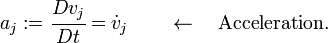
The resulting acceleration field is the material time derivative of the velocity
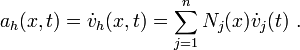
Hence,
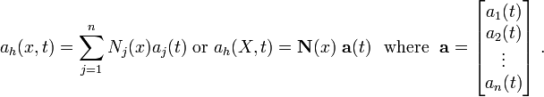
Note that the shape functions are functions of and not of . We
could transform them into function of using the inverse mapping
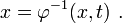
However, in that case the shape functions become functions of time and the procedure becomes more complicated.
The test (weighting) function is
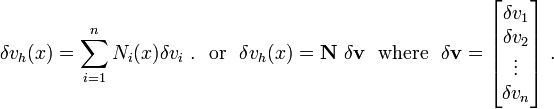
The derivatives of the test functions with respect to are

It is convenient to use the isoparametric concept to compute the spatial derivatives. Let us reexamine what this approach involves.
Figure 1 shows a two-noded 1-D element in the reference and current configurations along with the parent element.
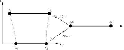 Figure 1. Reference and Current Configurations of a 1-D element. |
The map between the Eulerian coordinates and the parent coordinates is

At  ,
,

Therefore the displacement in the parent coordinates is
![u(\xi, t) = x(\xi, t) - x(\xi) = \mathbf{N}(\xi)~\left[\mathbf{x}^e(t) - \mathbf{X}^e\right]
\qquad \text{or}~~
{
u(\xi, t) = \mathbf{N}(\xi)~\mathbf{u}^e(t) ~.
}](../I/m/c8dc416e78a0517272d66bce67f916a4.png)
Similarly, the velocity and its variation in the parent coordinates are given by

The acceleration in the parent coordinates is given by
The rate of deformation is given by

We can evaluate the derivative with respect to by simply using the
map to the parent coordinate instead of mapping back to the reference
coordinates. Using the chain rule (for the two noded element)

In matrix form,

The rate of deformation in parent coordinates is then given by
To derive the finite element system of equations, we follow the usual approach of substituting the trial and test functions into the approximate weak form
![\int_{x_a}^{x_b} (\delta v_h)_{,x} (A~\sigma)~dx +
\int_{x_a}^{x_b}\delta v_h~\rho~A~\cfrac{Dv_h}{Dt}~dx =
\int_{x_a}^{x_b} \delta v_h~\rho~A~b~dx + \left[\delta v_h~A~\sigma\right]_{x_a}^{x_b} ~.](../I/m/571888e331170014c79f95326a1f9923.png)
Let us proceed term by term.
First LHS Term
The first term represents the virtual internal power
Plugging in the derivative of the test function, we get
![\begin{align}
\delta P_{\text{int}} & = \int_{x_a}^{x_b} \left[\sum_{i=1}^n N_{i,x}\delta v_i\right]
(A~\sigma)~dx\\
& = \sum_{i=1}^n \delta v_i
\left[\int_{x_a}^{x_b} N_{i,x}(A~\sigma)~dx\right]\\
& = \sum_{i=1}^n \delta v_i f_i^{\text{int}} ~.
\end{align}](../I/m/790ba5c76998613cd0c7fee318c86407.png)
The matrix form of the expression for virtual internal work is
The internal force is

Note that the above simplification only occurs in 1-D. In matrix form,

Remark:
Note that we can write
If we use the above relation, we get
Using the relation
we get
The above is the same as the expression we had for the internal force in the total Lagrangian formulation.
Second LHS Term
The second term represents the virtual kinetic power
Plugging in the test function, we get
![\begin{align}
\delta P_{\text{kin}}
& = \int_{x_a}^{x_b}\left[\sum_{i=1}^n \delta v_i N_i\right]
\rho~A~\cfrac{Dv_h}{Dt}~dx\\
& = \sum_{i=1}^n \delta v_i \left[\int_{x_a}^{x_b}
\rho~A~N_i~\cfrac{Dv_h}{Dt}~dx\right]\\
& = \sum_{i=1}^n \delta v_i f_i^{\text{kin}} ~.
\end{align}](../I/m/cce77557199195e5b23dfc163402bc8f.png)
The inertial (kinetic) force is
Now, plugging in the trial function into the expression for the inertial force, we get
![\begin{align}
f^{\text{kin}}_i
& = \int_{x_a}^{x_b}\rho~A~N_i
\left[\sum_{j=1}^n \cfrac{Dv_j}{Dt} N_j\right]~dx \\
& = \sum_{j=1}^n
\left[\int_{x_a}^{x_b}\rho~A~N_i~N_j~dx\right] \cfrac{Dv_j}{Dt} \\
& = \sum_{j=1}^n M_{ij} a_j
\end{align}](../I/m/6b96fe8ac977c5ed934e951fdfdb0f82.png)
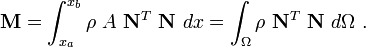
where

and
In matrix form,
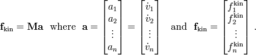
The consistent mass matrix in matrix notation is
Plugging the expression for the inertial force into the expression for virtual kinetic power, we get
![\begin{align}
\delta P_{\text{kin}}
& = \sum_{i=1}^n \delta v_i \left[\sum_{j=1}^n M_{ij} a_j\right] \\
& = \sum_{i=1}^n \sum_{j=1}^n \delta v_i M_{ij} a_j
\end{align}](../I/m/46c9a1dd3c4cfff3418c1ec8aee68862.png)
In matrix form,

Remark:
Note that since the integration domain is a function of time, the mass matrix for the updated Lagrangian formulation is also a function of time. However, from the conservation of mass, we have
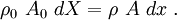
Therefore, we can write the mass matrix as

Hence the mass matrices are the same for both formulations.
RHS Terms
The right hand side terms represent the virtual external power
![\delta P_{\text{ext}} = \int_{x_a}^{x_b}\delta v_h~\rho~A~b~dx +
\left[\delta v_h~A~t_x\right]_{\Gamma_t}~.](../I/m/35190f91a776afb8064ef8432a72286c.png)
Plugging in the test function into the above expression gives
![\begin{align}
\delta P_{\text{ext}}
& = \int_{x_a}^{x_b}\left[\sum_{i=1}^n N_i~\delta v_i\right]\rho~A~b~dx +
\left[\left(\sum_{i=1}^n N_i~\delta v_i\right)
A~t_x\right]_{\Gamma_t} \\
& = \sum_{i=1}^n \delta v_i\left[\int_{x_a}^{x_b} N_i~\rho~A~b~dx\right] +
\left[\sum_{i=1}^n \delta v_i~N_i~A~t_X\right]_{\Gamma_t} \\
& = \sum_{i=1}^n \delta v_i\left[\int_{x_a}^{x_b} N_i~\rho~A~b~dx +
\left[N_i~A~t_x\right]_{\Gamma_t}\right] \\
& = \sum_{i=1}^n \delta v_i~f^{\text{ext}}_i ~.
\end{align}](../I/m/4914e6a7b011ee2ac55a5f319542277a.png)
In matrix notation,
The external force is given by
![{
f_i^{\text{ext}} =\int_{x_a}^{x_b} N_i~\rho~A~b~dx +
\left[N_i~A~t_x\right]_{\Gamma_t}~.
}](../I/m/dad0f8876a60bb4fa9eaea078b7fa626.png)
In matrix notation,
![{
\mathbf{f}_{\text{ext}} = \int_{x_a}^{x_b} \mathbf{N}^T~\rho~A~b~dx +
\left[\mathbf{N}^T~A~t_x\right]_{\Gamma_t}
}~~\text{or}~~
{
\mathbf{f}_{\text{ext}} = \int_{\Omega} \rho~\mathbf{N}^T~b~d\Omega +
\left[\mathbf{N}^T~A~t_x\right]_{\Gamma_t}~.
}](../I/m/9e9af7967035a3dbba0633c21158e5a7.png)
Remark:
Using the conservation of mass
and the relations between the traction sin the reference and the current configurations
we can transform the integral in the expression for the external force to one over the reference coordinates as follows:
![\mathbf{f}_{\text{ext}} = \int_{x_a}^{x_b} \mathbf{N}^T~\rho_0~A_0~b~dx +
\left[\mathbf{N}^T~A_0~t_x^0\right]_{\Gamma_t}~.](../I/m/8e30fde390739228a6ddc201f4b34316.png)
The above is the same as the expression we had for the external force in the total Lagrangian formulation.
Discrete Equations for Updated Lagrangian
The finite element equations in updated Lagrangian form are:
![{
\begin{align}
v(x,t) & = \sum_i N_i(x)~v_i^e(t) = \mathbf{N}~\mathbf{v}^e \\
D(x,t) & = \sum_i N_{i,x}~v_i^e(t) = \mathbf{B}~\mathbf{v}^e \\
\mathbf{f}^e_{\text{int}} & = \int_{\Omega^e} \mathbf{B}^T~\sigma~d\Omega \\
\mathbf{f}^e_{\text{ext}} & = \int_{\Omega^e} \rho~\mathbf{N}^T~b~d\Omega +
\left[\mathbf{N}^T~A~t_x \right]_{\Gamma_t^e} \\
\mathbf{M}^e & = \int_{\Omega_0^e}~\rho_0~\mathbf{N}^T~\mathbf{N}~d\Omega_0 \\
\mathbf{M}~\ddot{\mathbf{u}} & = \mathbf{f}_{\text{ext}} - \mathbf{f}_{\text{int}} ~.
\end{align}
}](../I/m/2e9145ae39bf81d5e5e4c6b43d664fe6.png)