Nonlinear finite elements/Total Lagrangian approach
< Nonlinear finite elementsTotal Lagrangian Approach
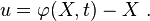
In the total Lagrangian approach, the discrete equations are formulated with respect to the reference configuration. The independent variables are  and
and  . The dependent variable is the displacement
  .
.
Total Lagrangian Stress and Strain Measures
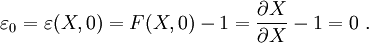
The strain is
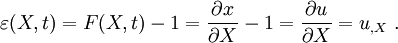
For the reference configuration,
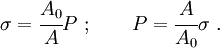
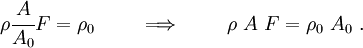
The Cauchy stress (force/current area) is

The engineering stress (force/initial area) is

The two stresses are related by
For the reference configuration,

Governing Equations in Total Lagrangian Form
The Total Lagrangian governing equations are:
- Conservation of Mass:
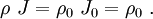
- For the axially loaded bar,
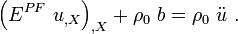
- Conservation of Momentum:
- For the bar
 is constant. Therefore,
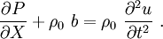
- In short form,
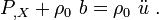
- If
 , we get the equilibrium equation
- Conservation of Energy:
- For the bar:
- In short form:
- Constitutive Equations:
- Total Form:
- For a linear elastic material:
![{
P(X,t) = E^{PF}~\varepsilon(X,t) =
E^{PF}~u_{,X} = E^{PF}\left[F(X,t) - 1\right]~.
}](../I/m/fe4a3d2cc7203d04d06c1e41d9579e34.png)
- The superscript
 refers to the fact that this function relates
  and
and  .
. - For small strains:
- Rate Form:
- For a linear elastic material:

The Wave Equation
The momentum equation is
The total form constitutive equation is

Plug constitutive equation into momentum equation to get
If  is constant in the bar and the body force is zero,
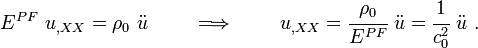
This is the wave equation (hyperbolic PDE). The wave speed is  .
If acceleration is zero, the equation becomes elliptic.
.
If acceleration is zero, the equation becomes elliptic.
Initial and Boundary Conditions
The governing equation for the rod is second-order in time. So two initial conditions are needed.
![{
\begin{align}
u(X,0) & = u_0(X) & ~\text{for}~ & X \in [0, L] \\
\dot{u}(X,0) & = v_0(X) & ~\text{for}~ & X \in [0, L]
\end{align}
}](../I/m/84fe2d7ad2f2748339a6ce53d46b97bf.png)
The rod is initially at rest. Therefore, the initial conditions are
![\begin{align}
u(X,0) & = 0 & ~\text{for}~ & X \in [0, L] \\
\dot{u}(X,0) & = 0 & ~\text{for}~ & X \in [0, L]
\end{align}](../I/m/91e6ed130392b11cf99b5b710923ba47.png)
Since the problem is one-dimensional, there are two boundary points.
Also, the momentum equation is second-order in the displacements.
Therefore, at each end, either  or
or  must be prescribed.
In mechanics, instead of , the traction is prescribed.
must be prescribed.
In mechanics, instead of , the traction is prescribed.
Let  be the part of the boundary where displacements are
prescribed. Let
be the part of the boundary where displacements are
prescribed. Let  be the part of the boundary where tractions
(force vector per unit area) are prescribed.
be the part of the boundary where tractions
(force vector per unit area) are prescribed.
Then the displacement boundary conditions are

The traction boundary conditions are

The unit normal to the boundary in the reference configuration is
 .
.
For the axially loaded bar, the displacement boundary condition is

The unit normal to the boundary is
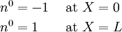
Therefore, the traction boundary condition is

For shock problems or fracture problems, an addition interior continuity or jump condition may be needed. This condition is written as

where

Weak Form for Total Lagrangian
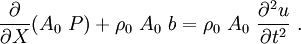
The momentum equation (in its full form) is

To get the weak form over an element, we multiply the equation by a
weighting function and integrate over the length of the element (from
 to
to  ).
).
![\int_{X_a}^{X_b} w\left[(A_0 P)_{,X} +
\rho_0 A_0 b - \rho_0 A_0 \ddot{u}\right]~dX = 0 ~.](../I/m/7d03046ffd78b473ca44e187a25cae0b.png)
Integrate the first term by parts to get
![\int_{X_a}^{X_b} w (A_0 P)_{,X}~dX = \left[w A_0 P\right]_{X_a}^{X_b} -
\int_{X_a}^{X_b} w_{,X} (A_0 P)~dX ~.](../I/m/ae43a2c2189e40ff42e63736b75fc079.png)
Plug the above into the weak form and rearrange to get
![\int_{X_a}^{X_b} w_{,X} (A_0 P)~dX + \int_{X_a}^{X_b} w\rho_0 A_0 \ddot{u}~dX =
\int_{X_a}^{X_b} w \rho_0 A_0 b~dX +\left[w A_0 P\right]_{X_a}^{X_b} ~.](../I/m/c62efb92e8397a1465dedb084a995201.png)
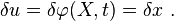
If we think of the weighting function  as a variation of that
satisfies the kinematic admissibility conditions, we get
as a variation of that
satisfies the kinematic admissibility conditions, we get
![{
\int_{X_a}^{X_b} (\delta u)_{,X} (A_0 P)~dX + \int_{X_a}^{X_b} \delta u\rho_0 A_0 \ddot{u}~dX =
\int_{X_a}^{X_b} \delta u \rho_0 A_0 b~dX +\left[\delta u A_0 P\right]_{X_a}^{X_b} ~.
}](../I/m/1e9424d8d76a1cd9511b5704cea1a57e.png)
Recall that
Therefore,
Taking a derivative of this variation, we have
Also,
![\begin{align}
\left[\delta u A_0 P\right]_{X_a}^{X_b} &=
[\delta u A_0 P]_{X_b} - [\delta u A_0 P]_{X_a} \\
&=[\delta u A_0 P n_0]_{X_b} + [\delta u A_0 P n_0]_{X_a} \\
&=[\delta u A_0 t^0_X]_{X_b} + [\delta u A_0 t^0_X]_{X_a} \\
&= \left[\delta u A_0 t^0_X\right]_{\Gamma_t} ~.
\end{align}](../I/m/7e82984f5e154c83f396b6298cd39728.png)
Therefore, we can alternatively write the weak form as
![{
\int_{X_a}^{X_b} \delta F A_0 P~dX + \int_{X_a}^{X_b} \delta u\rho_0 A_0 \ddot{u}~dX =
\int_{X_a}^{X_b} \delta u \rho_0 A_0 b~dX +\left[\delta u A_0 t^0_X\right]_{\Gamma_t}~.
}](../I/m/2bcc1fa592fddc3a2c70c31ba457b456.png)
Comparing with the energy equation, we see that the first term above is the internal virtual work and the weak form is the principle of virtual work for the 1-D problem. The weak form may also be written as

where,
![{
\begin{align}
\delta W_{\text{int}} & = \int_{X_a}^{X_b} (\delta u)_{,X} (A_0 P)~dX \\
\delta W_{\text{ext}} & = \int_{X_a}^{X_b} \delta u \rho_0 A_0 b~dX +
\left[\delta u A_0 P\right]_{X_a}^{X_b} \\
\delta W_{\text{kin}} & = \int_{X_a}^{X_b} \delta u\rho_0 A_0 \ddot{u}~dX
\end{align}
}](../I/m/d61bf7e919262f3c3a9fa972327eed5b.png)
Finite Element Discretization for Total Lagrangian
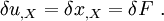
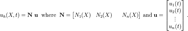
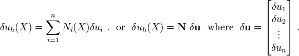
The trial solution is
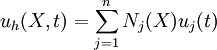
where  is the number of nodes. In matrix form,
The test (weighting) function is
The derivatives of the test functions with respect to are

We will derive the finite element system of equations after substituting these into the approximate weak form
![\int_{X_a}^{X_b} (\delta u_h)_{,X} (A_0 P)~dX + \int_{X_a}^{X_b} \delta u_h\rho_0 A_0 \ddot{u}_h~dX
=
\int_{X_a}^{X_b} \delta u_h \rho_0 A_0 b +\left[\delta u_h A_0 P\right]_{X_a}^{X_b} ~.](../I/m/6b813bf8364f61d48e309209c802fbad.png)
Let us proceed term by term.
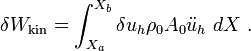
First LHS Term
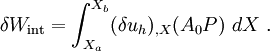
The first term represents the virtual internal work
Plugging in the derivative of the test function, we get
![\begin{align}
\delta W_{\text{int}} & = \int_{X_a}^{X_b} \left[\sum_{i=1}^n N_{i,X}\delta u_i\right]
(A_0 P)~dX\\
& = \sum_{i=1}^n \delta u_i
\left[\int_{X_a}^{X_b} N_{i,X} (A_0 P)~dX\right]\\
& = \sum_{i=1}^n \delta u_i f_i^{\text{int}} ~.
\end{align}](../I/m/5e46e384cd9392c29aa9903b64b949ad.png)
The last substitution is made because the virtual internal work is the work done by internal forces in moving through a virtual displacement. The matrix form of the expression for virtual internal work is
The internal force is

Second LHS Term
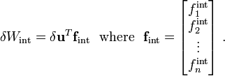
The second term represents the virtual kinetic work
Plugging in the test function, we get
![\begin{align}
\delta W_{\text{kin}}
& = \int_{X_a}^{X_b} \left[\sum_{i=1}^n \delta u_i N_i\right]
\rho_0 A_0 \ddot{u}_h~dX\\
& = \sum_{i=1}^n \delta u_i \left[\int_{X_a}^{X_b}
\rho_0 A_0 N_i \ddot{u}_h~dX\right]\\
& = \sum_{i=1}^n \delta u_i f_i^{\text{kin}} ~.
\end{align}](../I/m/3a4e995a43d4d73f05a02757e86cef8a.png)
The inertial (kinetic) force is
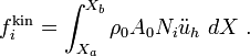
Now, plugging in the trial function into the expression for the inertial force, we get
![\begin{align}
f^{\text{kin}}_i
& = \int_{X_a}^{X_b} \rho_0 A_0 N_i
\left[\sum_{j=1}^n \ddot{u}_j N_j\right]~dX \\
& = \sum_{j=1}^n
\left[\int_{X_a}^{X_b} \rho_0 A_0 N_i N_j~dX\right] \ddot{u}_j \\
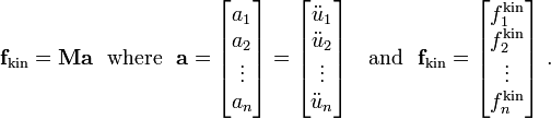
& = \sum_{j=1}^n M_{ij} a_j
\end{align}](../I/m/cd43b381e2a83348edaecb997b240ec9.png)
where

and

Note that the mass matrix is independent of time!
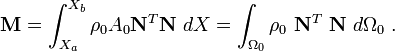
In matrix form,
The consistent mass matrix in matrix notation is
Plugging the expression for the inertial force into the expression for virtual kinetic work, we get
![\begin{align}
\delta W_{\text{kin}}
& = \sum_{i=1}^n \delta u_i \left[\sum_{j=1}^n M_{ij} a_j\right] \\
& = \sum_{i=1}^n \sum_{j=1}^n \delta u_i M_{ij} a_j
\end{align}](../I/m/4f4c7a4542a6a1fcbf5b4f483a154e82.png)
In matrix form,

RHS Terms
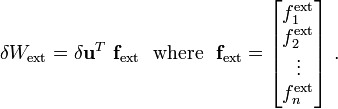
The right hand side terms represent the virtual external work
![\delta W_{\text{ext}} = \int_{X_a}^{X_b}\delta u_h\rho_0 A_0 b~dX +
\left[\delta u_h A_0 t^0_X\right]_{\Gamma_t}~.](../I/m/40acecf50608543da771639a5f7d8734.png)
Plugging in the test function into the above expression gives
![\begin{align}
\delta W_{\text{ext}}
& = \int_{X_a}^{X_b}\left[\sum_{i=1}^n N_i \delta u_i\right]\rho_0 A_0 b~dX +
\left[\left(\sum_{i=1}^n N_i \delta u_i\right)
A_0 t^0_X\right]_{\Gamma_t} \\
& = \sum_{i=1}^n \delta u_i \left[\int_{X_a}^{X_b} N_i \rho_0 A_0 b~dX\right] +
\left[\sum_{i=1}^n \delta u_i N_i A_0 t^0_X\right]_{\Gamma_t} \\
& = \sum_{i=1}^n \delta u_i \left[\int_{X_a}^{X_b} N_i \rho_0 A_0 b~dX +
\left[N_i A_0 t^0_X\right]_{\Gamma_t}\right] \\
& = \sum_{i=1}^n \delta u_i~f^{\text{ext}}_i ~.
\end{align}](../I/m/468fc321436779b9cad5fb06728942a0.png)
In matrix notation,
The external force is given by
![{
f_i^{\text{ext}} =\int_{X_a}^{X_b} N_i \rho_0 A_0 b~dX +
\left[N_i A_0 t^0_X\right]_{\Gamma_t}~.
}](../I/m/4a57aed9bfd422f2cc20911c7fa71099.png)
In matrix notation,
![{
\mathbf{f}_{\text{ext}} = \int_{X_a}^{X_b} \mathbf{N}^T \rho_0 A_0 b~dX +
\left[\mathbf{N}^T A_0 t^0_X\right]_{\Gamma_t}
}~~\text{or}~~
{
\mathbf{f}_{\text{ext}} = \int_{\Omega_0} \rho_0~\mathbf{N}^T~b~d\Omega_0 +
\left[\mathbf{N}^T A_0 t^0_X\right]_{\Gamma_t}~.
}](../I/m/6f5fcee60f985cb96f82f78a509b59c4.png)
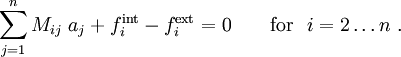
Collecting the terms, we get the finite element system of equations
![\sum_{i=1}^n \delta u_i \left[f_i^{\text{int}} + f_i^{\text{kin}} - f_i^{\text{ext}}\right]
= 0](../I/m/cb209fa64547cf70d8ef08555a3cc93f.png)
Now, the weighting function is arbitrary except at nodes where displacement BCs are prescribed. At these nodes the weighting function is zero.
For the bar, let us assume that a displacement is prescribed at node  .
Then, the finite element system of equations becomes
.
Then, the finite element system of equations becomes

or,
Since the displacement at node is known, the acceleration at node is
also known. Note that we have to differentiate the displacement twice
to get the acceleration and hence the prescribed displacement must be
a  function.
We can take the known acceleration  to the RHS to get
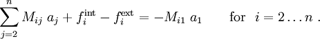
The above equation shows that prescribed boundary accelerations (and hence prescribed boundary displacements) contribute to nodes which are not on the boundary.
We can avoid that issue by making the mass matrix diagonal (using ad-hoc procedures that conserve momentum). If the mass matrix is diagonal, we get

In matrix form,

One way of generating a diagonal mass matrix or lumped mass matrix is the row-sum technique. The rows of the mass matrix are summed at lumped at the diagonal of the matrix. Thus,
![\begin{align}
M^{\text{diagonal}}_{ii}
& = \sum_{j=1}^n M^{\text{consistent}}_{ij} \\
& = \sum_{j=1}^n \int_{X_a}^{X_b} \rho_0 N_i N_j A_0 ~dX \\
& = \int_{X_a}^{X_b} \rho_0 N_i \left[\sum_{j=1}^n N_j\right] A_0 ~dX \\
& = \int_{X_a}^{X_b} \rho_0 N_i A_0 ~dX\qquad\text{since}~\sum_{j=1}^n N_j = 1~.
\end{align}](../I/m/f1d2d00b8a8fa8cf4a75bdad8bb9832a.png)
Discrete Equations for Total Lagrangian
The finite element equations in total Lagrangian form are:
![{
\begin{align}
u(X,t) & = \sum_i N_i(X)~u_i^e(t) = \mathbf{N}~\mathbf{u}^e \\
\varepsilon(X,t) & = \sum_i N_{i,X}~u_i^e(t) = \mathbf{B}_0~\mathbf{u}^e \\
F(X,t) & = \sum_i N_{i,X}~x_i^e(t) = \mathbf{B}_0~\mathbf{x}^e \\
\mathbf{f}^e_{\text{int}} & = \int_{\Omega_0^e} \mathbf{B}_0^T P~d\Omega_0 \\
\mathbf{f}^e_{\text{ext}} & = \int_{\Omega_0^e} \rho_0 \mathbf{N}^Tb~d\Omega_0 +
\left[\mathbf{N}^T A_0 t_X^0 \right]_{\Gamma_t^e} \\
\mathbf{M}^e & = \int_{\Omega_0^e} \rho_0 \mathbf{N}^T \mathbf{N} ~d\Omega_0 \\
\mathbf{M}~\ddot{\mathbf{u}} & = \mathbf{f}_{\text{ext}} - \mathbf{f}_{\text{int}} ~.
\end{align}
}](../I/m/e2bb7972d102c6b8322de2b4079efebb.png)