Introduction to Elasticity/Tensors
< Introduction to ElasticityTensors in Solid Mechanics
A sound understanding of tensors and tensor operation is essential if you want to read and understand modern papers on solid mechanics and finite element modeling of complex material behavior. This brief introduction gives you an overview of tensors and tensor notation. For more details you can read A Brief on Tensor Analysis by J. G. Simmonds, the appendix on vector and tensor notation from Dynamics of Polymeric Liquids - Volume 1 by R. B. Bird, R. C. Armstrong, and O. Hassager, and the monograph by R. M. Brannon. An introduction to tensors in continuum mechanics can be found in An Introduction to Continuum Mechanics by M. E. Gurtin. Most of the material in this page is based on these sources.
Notation
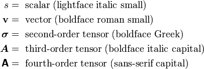
The following notation is usually used in the literature:
Motivation
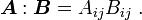
A force  has a magnitude and a direction, can be added to another force, be multiplied by a scalar and so on. These properties make the force a vector.
Similarly, the displacement  is a vector because it can be added to other displacements and satisfies the other properties of a vector.
However, a force cannot be added to a displacement to yield a physically meaningful quantity. So the physical spaces that these two quantities lie on must be different.
Recall that a constant force  moving through a displacement
  does
does  units of work. How do we compute this product when the spaces of and are different? If you try to compute the product on a graph, you will have to convert both quantities to a single basis and then compute the scalar product.
An alternative way of thinking about the operation is to think of as a linear operator that acts on to produce a scalar quantity (work). In the notation of sets we can write

A first order tensor is a linear operator that sends vectors to scalars.
Next, assume that the force acts at a point  . The moment of the force about the origin is given by
  which is a vector. The vector product can be thought of as an linear operation too. In this case the effect of the operator is to convert a vector into another vector.
A second order tensor is a linear operator that sends vectors to vectors.
According to Simmonds, "the name tensor comes from elasticity theory where in a loaded elastic body the stress tensor acting on a unit vector normal to a plane through a point delivers the tension (i.e., the force per unit area) acting across the plane at that point."
Examples of second order tensors are the stress tensor, the deformation gradient tensor, the velocity gradient tensor, and so on.
Another type of tensor that we encounter frequently in mechanics is the fourth order tensor that takes strains to stresses. In elasticity, this is the stiffness tensor.
A fourth order tensor is a linear operator that sends second order tensors to second order tensors.
Tensor algebra
A tensor  is a linear transformation from a vector space
  to . Thus, we can write

More often, we use the following notation:

I have used the "dot" notation in this handout. None of the above notations is obviously superior to the others and each is used widely.
Addition of tensors
Let and  be two tensors. Then the sum
  is another tensor
  defined by

Multiplication of a tensor by a scalar
Let be a tensor and let  be a scalar. Then the product
  is a tensor defined by

Zero tensor
The zero tensor  is the tensor which maps every vector
  into the zero vector.

Identity tensor
The identity tensor  takes every vector into itself.

The identity tensor is also often written as  .
.
Product of two tensors
Let and be two tensors. Then the product  is the tensor that is defined by

In general 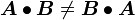 .
.
Transpose of a tensor
The transpose of a tensor is the unique tensor  defined by

The following identities follow from the above definition:
Symmetric and skew tensors
A tensor is symmetric if

A tensor is skew if

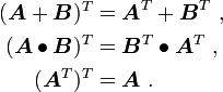
Every tensor can be expressed uniquely as the sum of a symmetric tensor  (the symmetric part of ) and a skew tensor
  (the skew part of ).
Tensor product of two vectors
The tensor (or dyadic) product  (also written
  ) of two vectors
  and
and  is a tensor that assigns to each vector the vector
  .
.

Notice that all the above operations on tensors are remarkably similar to matrix operations.
Spectral theorem
The spectral theorem for tensors is widely used in mechanics. We will start off by definining eigenvalues and eigenvectors.
Eigenvalues and eigenvectors
Let  be a second order tensor. Let
  be a scalar and
  be a vector such that

Then is called an eigenvalue of and is an eigenvector .
A second order tensor has three eigenvalues and three eigenvectors, since the space is three-dimensional. Some of the eigenvalues might be repeated. The number of times an eigenvalue is repeated is called multiplicity.
In mechanics, many second order tensors are symmetric and positive definite. Note the following important properties of such tensors:
- If is positive definite, then
 .
. - If is symmetric, the eigenvectors are mutually orthogonal.
For more on eigenvalues and eigenvectors see Applied linear operators and spectral methods.
|
Let
This relation is called the spectral decomposition of |
 form an orthonormal basis.
 are the corresponding eigenvalues then
 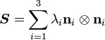 .
.Polar decomposition theorem
Let  be second order tensor with
  . Then
- there exist positive definite, symmetric tensors
 ,
, and a rotation (orthogonal) tensor
  such that
  .
. - also each of these decompositions is unique.
Principal invariants of a tensor
Let  be a second order tensor. Then the determinant of
  can be expressed as

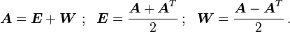
The quantities  are called the principal invariants of . Expressions of the principal invariants are given below.
|
Principal invariants of |
![\begin{align}
I_1 & = \text{tr}~ \boldsymbol{S} = \lambda_1 + \lambda_2 + \lambda_3 \\
I_2 & = \cfrac{1}{2}\left[ (\text{tr}~ \boldsymbol{S})^2 - \text{tr}(\boldsymbol{S^2})\right] = \lambda_1~\lambda_2 + \lambda_2~\lambda_3 + \lambda_3~\lambda_1\\
I_3 & = \det\boldsymbol{S} = \lambda_1~\lambda_2~\lambda_3
\end{align}](../I/m/4a473f8de799a8e516ec11120f6cf75a.png)
Note that is an eigenvalue of if and only if
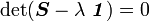
The resulting equations is called the characteristic equation and is usually written in expanded form as

Cayley-Hamilton theorem
The Cayley-Hamilton theorem is a very useful result in continuum mechanics. It states that
|
Cayley-Hamilton theorem If |

Index notation
All the equations so far have made no mention of the coordinate system. When we use vectors and tensor in computations we have to express them in some coordinate system (basis) and use the components of the object in that basis for our computations.
Commonly used bases are the Cartesian coordinate frame, the cylindrical coordinate frame, and the spherical coordinate frame.
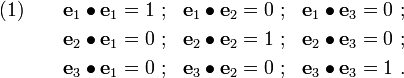
A Cartesian coordinate frame consists of an orthonormal basis  together with a point
  called the origin. Since these vectors are mutually perpendicular, we have the following relations:
Kronecker delta
To make the above relations more compact, we introduce the Kronecker delta symbol
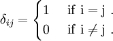
Then, instead of the nine equations in (1) we can write (in index notation)
Einstein summation convention
Recall that the vector can be written as
In index notation, equation (2) can be written as

This convention is called the Einstein summation convention. If indices are repeated, we understand that to mean that there is a sum over the indices.
Components of a vector
We can write the Cartesian components of a vector in the basis as

Components of a tensor
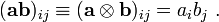
Similarly, the components of  of a tensor are defined by
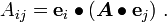
Using the definition of the tensor product, we can also write
Using the summation convention,

In this case, the bases of the tensor are  and the components are .
Operation of a tensor on a vector
From the definition of the components of tensor , we can also see that (using the summation convention)

Dyadic product
Similarly, the dyadic product can be expressed as
Matrix notation
We can also write a tensor  in matrix notation as
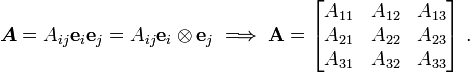
Note that the Kronecker delta represents the components of the identity tensor in a Cartesian basis. Therefore, we can write
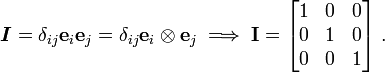
Tensor inner product
The inner product  of two tensors and is an operation that generates a scalar. We define (summation implied)
The inner product can also be expressed using the trace :

Proof using the definition of the trace below :


Trace of a tensor
The trace of a tensor is the scalar given by

(** Needs a proper definition **)
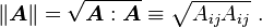
Magnitude of a tensor
The magnitude of a tensor is defined by
Tensor product of a tensor with a vector
Another tensor operation that is often seen is the tensor product of a tensor with a vector. Let be a tensor and let be a vector. Then the tensor cross product gives a tensor defined by

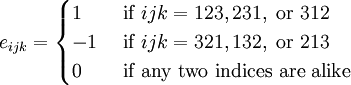
Permutation symbol
The permutation symbol  is defined as
Identities in tensor algebra
Let ,  and
and  be three second order tensors. Then

Proof:
It is easiest to show these relations by using index notation with respect to an orthonormal basis. Then we can write
Similarly,


Tensor calculus
Recall that the vector differential operator (with respect to a Cartesian basis) is defined as
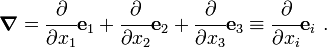
In this section we summarize some operations of  on vectors and tensors.
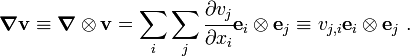
The gradient of a vector field
The dyadic product  (or
(or  ) is called the gradient of the vector field . Therefore, the quantity
  is a tensor given by
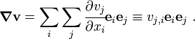
In the alternative dyadic notation,
'Warning: Some authors define the  component of as
 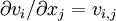 .
.
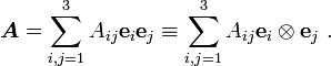
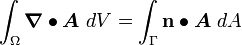
The divergence of a tensor field
Let be a tensor field. Then the divergence of the tensor field is a vector  given by
![{
\boldsymbol{\nabla}\bullet{\boldsymbol{A}} = \sum_j \left[\sum_i \cfrac{\partial A_{ij}}{\partial x_i}\right] \mathbf{e}_j
\equiv \cfrac{\partial A_{ij}}{\partial x_i} \mathbf{e}_j = A_{ij,i} \mathbf{e}_j~.
}](../I/m/d678711d2ad6eb578cc9ff39915c9e61.png)
To fix the definition of divergence of a general tensor field (possibly of higher order than 2), we use the relation

where  is an arbitrary constant vector.
The Laplacian of a vector field
The Laplacian of a vector field is given by
![{
\nabla^2{\mathbf{v}} = \boldsymbol{\nabla}\bullet{\boldsymbol{\nabla}{\mathbf{v}}} =
\sum_j \left[\sum_i \cfrac{\partial^2 v_j}{\partial x_i^2}\right] \mathbf{e}_j \equiv
v_{j,ii} \mathbf{e}_j ~.
}](../I/m/7ea9a7d91f99b09a81b524a79c7553f7.png)
Tensor Identities
Some important identities involving tensors are:
 .
. .
. .
. .
. .
. .
.
Integral theorems
The following integral theorems are useful in continuum mechanics and finite elements.
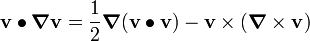
The Gauss divergence theorem
If  is a region in space enclosed by a surface
  and is a tensor field, then
where  is the unit outward normal to the surface.
The Stokes curl theorem
If is a surface bounded by a closed curve  , then
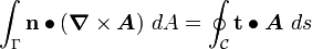
where is a tensor field, is the unit normal vector to in the direction of a right-handed screw motion along , and  is a unit tangential vector in the direction of integration along .
The Leibniz formula
Let be a closed moving region of space enclosed by a surface . Let the velocity of any surface element be . Then if  is a tensor function of position and time,
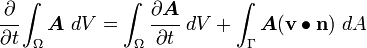
where is the outward unit normal to the surface .
Directional derivatives
We often have to find the derivatives of vectors with respect to vectors and of tensors with respect to vectors and tensors. The directional directive provides a systematic way of finding these derivatives.
The definitions of directional derivatives for various situations are given below. It is assumed that the functions are sufficiently smooth that derivatives can be taken.
Derivatives of scalar valued functions of vectors
Let  be a real valued function of the vector
  . Then the
derivative of with respect to (or at ) in the direction
is the vector defined as
. Then the
derivative of with respect to (or at ) in the direction
is the vector defined as
![\frac{\partial f}{\partial \mathbf{v}}\cdot\mathbf{u} = Df(\mathbf{v})[\mathbf{u}]
= \left[\frac{\partial }{\partial \alpha}~f(\mathbf{v} + \alpha~\mathbf{u})\right]_{\alpha = 0}](../I/m/f8fb9fb99907af980cfd82f9a6dbb256.png)
for all vectors .
Properties:
1) If 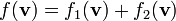 then
then 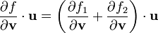
2) If 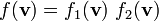 then
then 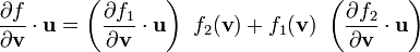
3) If 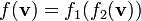 then
then 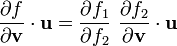
Derivatives of vector valued functions of vectors
Let  be a vector valued function of the vector . Then the
derivative of with respect to (or at ) in the direction
is the second order tensor defined as
be a vector valued function of the vector . Then the
derivative of with respect to (or at ) in the direction
is the second order tensor defined as
![\frac{\partial \mathbf{f}}{\partial \mathbf{v}}\cdot\mathbf{u} = D\mathbf{f}(\mathbf{v})[\mathbf{u}]
= \left[\frac{\partial }{\partial \alpha}~\mathbf{f}(\mathbf{v} + \alpha~\mathbf{u})\right]_{\alpha = 0}](../I/m/f7d996582b85604b0a27bfd469b80f73.png)
for all vectors .
Properties:
1) If 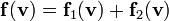 then
then 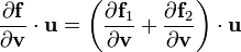
2) If 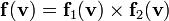 then
then 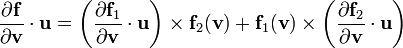
3) If  then
then 
Derivatives of scalar valued functions of tensors
Let  be a real valued function of the second order tensor . Then
the derivative of with respect to (or at ) in the direction
be a real valued function of the second order tensor . Then
the derivative of with respect to (or at ) in the direction
 is the second order tensor defined as
![\frac{\partial f}{\partial \boldsymbol{S}}:\boldsymbol{T} = Df(\boldsymbol{S})[\boldsymbol{T}]
= \left[\frac{\partial }{\partial \alpha}~f(\boldsymbol{S} + \alpha~\boldsymbol{T})\right]_{\alpha = 0}](../I/m/5c992312964fa4501c7b6bce099a19d3.png)
for all second order tensors .
Properties:
1) If  then
then 
2) If 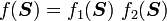 then
then 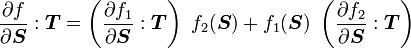
3) If 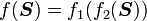 then
then 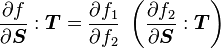
Derivatives of tensor valued functions of tensors
Let  be a second order tensor valued function of the second order
tensor . Then the derivative of with respect to
(or at ) in the direction is the fourth order tensor defined as
be a second order tensor valued function of the second order
tensor . Then the derivative of with respect to
(or at ) in the direction is the fourth order tensor defined as
![\frac{\partial \boldsymbol{F}}{\partial \boldsymbol{S}}:\boldsymbol{T} = D\boldsymbol{F}(\boldsymbol{S})[\boldsymbol{T}]
= \left[\frac{\partial }{\partial \alpha}~\boldsymbol{F}(\boldsymbol{S} + \alpha~\boldsymbol{T})\right]_{\alpha = 0}](../I/m/f93d6147cdd5a47ed969e247fe953f64.png)
for all second order tensors .
Properties:
1) If 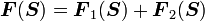 then
then 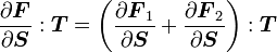
2) If 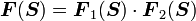 then
then 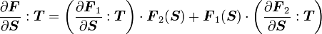
3) If 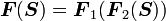 then
then 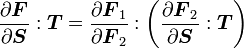
3) If 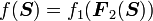 then
then 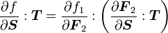
Derivative of the determinant of a tensor
|
Derivative of the determinant of a tensor The derivative of the determinant of a second order tensor In an orthonormal basis the components of |
![\frac{\partial }{\partial \boldsymbol{A}}\det(\boldsymbol{A}) = \det(\boldsymbol{A})~[\boldsymbol{A}^{-1}]^T ~.](../I/m/6f4279849cd49175f296245bc72e8e8f.png)
 . In that case, the right hand side corresponds the
cofactors of the matrix.
. In that case, the right hand side corresponds the
cofactors of the matrix.Proof:
Let
. Then, from the definition of the derivative of a scalar valued function of a tensor, we have
Recall that we can expand the determinant of a tensor in the form of a characteristic equation in terms of the invariants
using (note the sign of
Using this expansion we can write
Recall that the invariant
is given by
Hence,
Invoking the arbitrariness of
![\begin{align}
\frac{\partial f}{\partial \boldsymbol{A}}:\boldsymbol{T} & =
\left.\cfrac{d}{d\alpha} \det(\boldsymbol{A} + \alpha~\boldsymbol{T}) \right|_{\alpha=0} \\
& = \left.\cfrac{d}{d\alpha}
\det\left[\alpha~\boldsymbol{A}\left(\cfrac{1}{\alpha}~\boldsymbol{\mathit{1}} + \boldsymbol{A}^{-1}\cdot\boldsymbol{T}\right)
\right] \right|_{\alpha=0} \\
& = \left.\cfrac{d}{d\alpha} \left[\alpha^3~\det(\boldsymbol{A})~
\det\left(\cfrac{1}{\alpha}~\boldsymbol{\mathit{1}} + \boldsymbol{A}^{-1}\cdot\boldsymbol{T}\right)\right]
\right|_{\alpha=0} ~.
\end{align}](../I/m/90e63d233f3540c3bfacd72b81a82996.png)

![\begin{align}
\frac{\partial f}{\partial \boldsymbol{A}}:\boldsymbol{T}
& = \left.\cfrac{d}{d\alpha} \left[\alpha^3~\det(\boldsymbol{A})~
\left(\cfrac{1}{\alpha^3} + I_1(\boldsymbol{A}^{-1}\cdot\boldsymbol{T})~\cfrac{1}{\alpha^2} +
I_2(\boldsymbol{A}^{-1}\cdot\boldsymbol{T})~\cfrac{1}{\alpha} + I_3(\boldsymbol{A}^{-1}\cdot\boldsymbol{T})\right)
\right] \right|_{\alpha=0} \\
& = \left.\det(\boldsymbol{A})~\cfrac{d}{d\alpha} \left[
1 + I_1(\boldsymbol{A}^{-1}\cdot\boldsymbol{T})~\alpha +
I_2(\boldsymbol{A}^{-1}\cdot\boldsymbol{T})~\alpha^2 + I_3(\boldsymbol{A}^{-1}\cdot\boldsymbol{T})~\alpha^3
\right] \right|_{\alpha=0} \\
& = \left.\det(\boldsymbol{A})~\left[I_1(\boldsymbol{A}^{-1}\cdot\boldsymbol{T}) +
2~I_2(\boldsymbol{A}^{-1}\cdot\boldsymbol{T})~\alpha + 3~I_3(\boldsymbol{A}^{-1}\cdot\boldsymbol{T})~\alpha^2
\right] \right|_{\alpha=0} \\
& = \det(\boldsymbol{A})~I_1(\boldsymbol{A}^{-1}\cdot\boldsymbol{T}) ~.
\end{align}](../I/m/9877d64b2d13c6f03da7a9451db28530.png)
![\frac{\partial f}{\partial \boldsymbol{A}}:\boldsymbol{T} = \det(\boldsymbol{A})~\text{tr}(\boldsymbol{A}^{-1}\cdot\boldsymbol{T})
= \det(\boldsymbol{A})~[\boldsymbol{A}^{-1}]^T : \boldsymbol{T} ~.](../I/m/a96247bfbfae89c3c2158816e9d0a797.png)
![\frac{\partial f}{\partial \boldsymbol{A}} = \det(\boldsymbol{A})~[\boldsymbol{A}^{-1}]^T ~.](../I/m/e4d84ff1d98ff7ab1c84de1868388458.png)
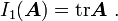
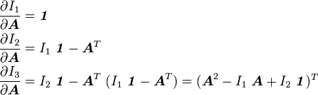
Derivatives of the invariants of a tensor
|
Derivatives of the principal invariants of a tensor The principal invariants of a second order tensor are The derivatives of these three invariants with respect to |
![\begin{align}
I_1(\boldsymbol{A}) & = \text{tr}{\boldsymbol{A}} \\
I_2(\boldsymbol{A}) & = \frac{1}{2} \left[ (\text{tr}{\boldsymbol{A}})^2 - \text{tr}{\boldsymbol{A}^2} \right] \\
I_3(\boldsymbol{A}) & = \det(\boldsymbol{A})
\end{align}](../I/m/e031982dab936e06aca3ce79d09dd9f2.png)
![\begin{align}
\frac{\partial I_1}{\partial \boldsymbol{A}} & = \boldsymbol{\mathit{1}} \\
\frac{\partial I_2}{\partial \boldsymbol{A}} & = I_1~\boldsymbol{\mathit{1}} - \boldsymbol{A}^T \\
\frac{\partial I_3}{\partial \boldsymbol{A}} & = \det(\boldsymbol{A})~[\boldsymbol{A}^{-1}]^T
= I_2~\boldsymbol{\mathit{1}} - \boldsymbol{A}^T~(I_1~\boldsymbol{\mathit{1}} - \boldsymbol{A}^T)
= (\boldsymbol{A}^2 - I_1~\boldsymbol{A} + I_2~\boldsymbol{\mathit{1}})^T
\end{align}](../I/m/462342e42fb5fc294822baa2b32ff616.png)
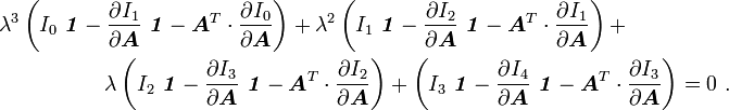
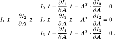
Proof:
From the derivative of the determinant we know that
For the derivatives of the other two invariants, let us go back to the characteristic equation
Using the same approach as for the determinant of a tensor, we can show that
Now the left hand side can be expanded as
Hence
or,
Expanding the right hand side and separating terms on the left hand side gives
or,
If we define
and
, we can write the above as
Collecting terms containing various powers of
Then, invoking the arbitrariness of
This implies that
![\frac{\partial I_3}{\partial \boldsymbol{A}} = \det(\boldsymbol{A})~[\boldsymbol{A}^{-1}]^T ~.](../I/m/3dba07872f4d2762f050eb4bfa0f2d3f.png)
![\frac{\partial }{\partial \boldsymbol{A}}\det(\lambda~\boldsymbol{\mathit{1}} + \boldsymbol{A}) =
\det(\lambda~\boldsymbol{\mathit{1}} + \boldsymbol{A})~[(\lambda~\boldsymbol{\mathit{1}}+\boldsymbol{A})^{-1}]^T ~.](../I/m/f4c1bc679081c1ff24ea1b327e861013.png)
![\begin{align}
\frac{\partial }{\partial \boldsymbol{A}}\det(\lambda~\boldsymbol{\mathit{1}} + \boldsymbol{A}) & =
\frac{\partial }{\partial \boldsymbol{A}}\left[
\lambda^3 + I_1(\boldsymbol{A})~\lambda^2 + I_2(\boldsymbol{A})~\lambda + I_3(\boldsymbol{A}) \right] \\
& =
\frac{\partial I_1}{\partial \boldsymbol{A}}~\lambda^2 + \frac{\partial I_2}{\partial \boldsymbol{A}}~\lambda +
\frac{\partial I_3}{\partial \boldsymbol{A}}~.
\end{align}](../I/m/0cccee2c6790ad09f86a08f7d515f21c.png)
![\frac{\partial I_1}{\partial \boldsymbol{A}}~\lambda^2 + \frac{\partial I_2}{\partial \boldsymbol{A}}~\lambda +
\frac{\partial I_3}{\partial \boldsymbol{A}} =
\det(\lambda~\boldsymbol{\mathit{1}} + \boldsymbol{A})~[(\lambda~\boldsymbol{\mathit{1}}+\boldsymbol{A})^{-1}]^T](../I/m/d1a88c6a225f551f7c68b321095f2de4.png)
![(\lambda~\boldsymbol{\mathit{1}}+\boldsymbol{A})^T\cdot\left[
\frac{\partial I_1}{\partial \boldsymbol{A}}~\lambda^2 + \frac{\partial I_2}{\partial \boldsymbol{A}}~\lambda +
\frac{\partial I_3}{\partial \boldsymbol{A}}\right] =
\det(\lambda~\boldsymbol{\mathit{1}} + \boldsymbol{A})~\boldsymbol{\mathit{1}} ~.](../I/m/d99fe1fc70f607dca5765ec2190fc027.png)
![(\lambda~\boldsymbol{\mathit{1}} +\boldsymbol{A}^T)\cdot\left[
\frac{\partial I_1}{\partial \boldsymbol{A}}~\lambda^2 + \frac{\partial I_2}{\partial \boldsymbol{A}}~\lambda +
\frac{\partial I_3}{\partial \boldsymbol{A}}\right] =
\left[\lambda^3 + I_1~\lambda^2 + I_2~\lambda + I_3\right]
\boldsymbol{\mathit{1}}](../I/m/89df0f22b98b33ed82ca716de7a9b37b.png)
![\begin{align}
\left[\frac{\partial I_1}{\partial \boldsymbol{A}}~\lambda^3 \right.&
\left.+ \frac{\partial I_2}{\partial \boldsymbol{A}}~\lambda^2 +
\frac{\partial I_3}{\partial \boldsymbol{A}}~\lambda\right]\boldsymbol{\mathit{1}} +
\boldsymbol{A}^T\cdot\frac{\partial I_1}{\partial \boldsymbol{A}}~\lambda^2 +
\boldsymbol{A}^T\cdot\frac{\partial I_2}{\partial \boldsymbol{A}}~\lambda +
\boldsymbol{A}^T\cdot\frac{\partial I_3}{\partial \boldsymbol{A}} \\
& =
\left[\lambda^3 + I_1~\lambda^2 + I_2~\lambda + I_3\right]
\boldsymbol{\mathit{1}} ~.
\end{align}](../I/m/c388c8b7cc3c8fad584f8ac00da12fe4.png)
![\begin{align}
\left[\frac{\partial I_1}{\partial \boldsymbol{A}}~\lambda^3 \right.&
\left.+ \frac{\partial I_2}{\partial \boldsymbol{A}}~\lambda^2 +
\frac{\partial I_3}{\partial \boldsymbol{A}}~\lambda + \frac{\partial I_4}{\partial \boldsymbol{A}}\right]\boldsymbol{\mathit{1}} +
\boldsymbol{A}^T\cdot\frac{\partial I_0}{\partial \boldsymbol{A}}~\lambda^3 +
\boldsymbol{A}^T\cdot\frac{\partial I_1}{\partial \boldsymbol{A}}~\lambda^2 +
\boldsymbol{A}^T\cdot\frac{\partial I_2}{\partial \boldsymbol{A}}~\lambda +
\boldsymbol{A}^T\cdot\frac{\partial I_3}{\partial \boldsymbol{A}} \\
&=
\left[I_0~\lambda^3 + I_1~\lambda^2 + I_2~\lambda + I_3\right]
\boldsymbol{\mathit{1}} ~.
\end{align}](../I/m/04fbec4739fd8c111c00fb290a91b288.png)
Derivative of the identity tensor
Let  be the second order identity tensor. Then the derivative of this
tensor with respect to a second order tensor is given by
be the second order identity tensor. Then the derivative of this
tensor with respect to a second order tensor is given by

This is because is independent of .
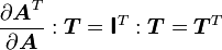
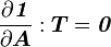
Derivative of a tensor with respect to itself
Let be a second order tensor. Then
![\frac{\partial \boldsymbol{A}}{\partial \boldsymbol{A}}:\boldsymbol{T} = \left[\frac{\partial }{\partial \alpha} (\boldsymbol{A} + \alpha~\boldsymbol{T})\right]_{\alpha = 0} = \boldsymbol{T} = \boldsymbol{\mathsf{I}}:\boldsymbol{T}](../I/m/f0ddf5fa18e025f6ee5bcd9f6a04cbcb.png)
Therefore,

Here  is the fourth order identity tensor. In index
notation with respect to an orthonormal basis
is the fourth order identity tensor. In index
notation with respect to an orthonormal basis

This result implies that
where

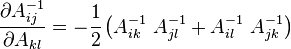
Therefore, if the tensor is symmetric, then the derivative is also symmetric and
we get
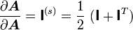
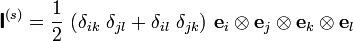
where the symmetric fourth order identity tensor is
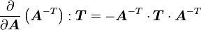
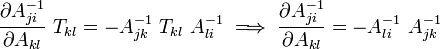
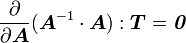
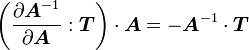
Derivative of the inverse of a tensor
|
Derivative of the inverse of a tensor Let In index notation with respect to an orthonormal basis We also have In index notation If the tensor |
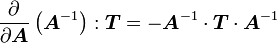
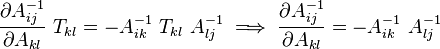
Proof:
Recall that
Since
, we can write
Using the product rule for second order tensors
we get
or,
Therefore,
![\frac{\partial }{\partial \boldsymbol{S}}[\boldsymbol{F}_1(\boldsymbol{S})\cdot\boldsymbol{F}_2(\boldsymbol{S})]:\boldsymbol{T} =
\left(\frac{\partial \boldsymbol{F}_1}{\partial \boldsymbol{S}}:\boldsymbol{T}\right)\cdot\boldsymbol{F}_2 +
\boldsymbol{F}_1\cdot\left(\frac{\partial \boldsymbol{F}_2}{\partial \boldsymbol{S}}:\boldsymbol{T}\right)](../I/m/c5834120647d610a8ffede8fe59d9e6e.png)

Remarks
The boldface notation that I've used is called the Gibbs notation. The index notation that I have used is also called Cartesian tensor notation.