Nonlinear finite elements/Steady state heat conduction

Subject classification: this is a physics resource .

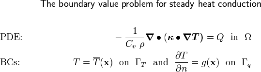
Steady state heat conduction

If the problem does not depend on time and the material is isotropic, we get the boundary value problem for steady state heat conduction.

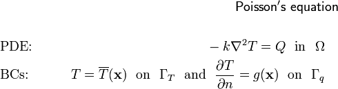
 ${ \begin{align} & &\mathsf{ The~ boundary~ value~ problem ~for~ steady~ heat ~conduction}\\ & & \\ & \text{PDE:}~~~ &~~~- \frac{1}{C_v~\rho} \boldsymbol{\nabla} \bullet (\boldsymbol{\kappa}\bullet\boldsymbol{\nabla T)} = Q ~~\text{in}~~\Omega\quad\\ & \text{BCs:}~~~ &~~~ T = \overline{T}(\mathbf{x})~~\text{on}~~\Gamma_T ~~\text{and}~~ \frac{\partial T}{\partial n} = g(\mathbf{x})~~\text{on}~~\Gamma_q\quad\\ \end{align} }$

Poisson's equation

If the material is homogeneous the density, heat capacity, and the thermal conductivity are constant. Define the thermal diffusivity as

k := \frac{\kappa}{C_v~\rho}

Then, the boundary value problem becomes

 ${ \begin{align} & &\mathsf{ Poisson's~ equation}\\ & & \\ & \text{PDE:}~~~ &~~~- k \nabla^2 T = Q ~~\text{in}~~\Omega\quad\\ & \text{BCs:}~~~ &~~~ T = \overline{T}(\mathbf{x})~~\text{on}~~\Gamma_T ~~\text{and}~~ \frac{\partial T}{\partial n} = g(\mathbf{x})~~\text{on}~~\Gamma_q\quad\\ \end{align} }$

where $\nabla^2 T$ is the Laplacian

\nabla^2 T := \boldsymbol{\nabla} \bullet \boldsymbol{\nabla T}

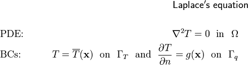
Laplace's equation

Finally, if there is no internal source of heat, the value of $Q$ is zero, and we get Laplace's equation.

 ${ \begin{align} & &\mathsf{ Laplace's~ equation}\\ & & \\ & \text{PDE:}~~~ &~~~\nabla^2 T = 0 ~~\text{in}~~\Omega\quad\\ & \text{BCs:}~~~ &~~~ T = \overline{T}(\mathbf{x})~~\text{on}~~\Gamma_T ~~\text{and}~~ \frac{\partial T}{\partial n} = g(\mathbf{x})~~\text{on}~~\Gamma_q\quad\\ \end{align} }$

The Analogous Membrane Problem

The thin elastic membrane problem is another similar problem. See Figure 1 for the geometry of the membrane.

The membrane is thin and elastic. It is initially planar and occupies the 2D domain $\Omega$ . It is fixed along part of its boundary $\Gamma_u$ . A transverse force $\mathbf{f}$ per unit area is applied. The final shape at equilibrium is nonplanar. The final displacement of a point $\mathbf{x}$ on the membrane is $\mathbf{u}(\mathbf{x})$ . There is no dependence on time.

The goal is to find the displacement $\mathbf{u}(\mathbf{x})$ at equilibrium.

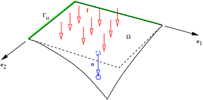Figure 1. The membrane problem.

It turns out that the equations for this problem are the same as those for the heat conduction problem - with the following changes:

The time derivatives vanish.
The balance of energy is replaced by the balance of forces.
The constitutive equation is replaced by a relation that states that the vertical force depends on the displacement gradient ( $\boldsymbol{\nabla} \mathbf{u}$ ).

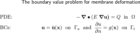
If the membrane if inhomogeneous, the boundary value problem is:

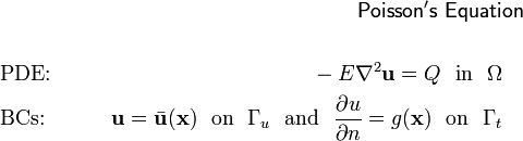
 ${ \begin{align} & &\mathsf{ The~boundary~ value~ problem~ for~ membrane~ deformation}\\ & & \\ & \text{PDE:}~~~ &~~~- \boldsymbol{\nabla} \bullet (E~\boldsymbol{\nabla \mathbf{u})} = Q ~~\text{in}~~\Omega\quad\\ & \text{BCs:}~~~ &~~~ \mathbf{u} = \bar{\mathbf{u}}(\mathbf{x})~~\text{on}~~\Gamma_u ~~\text{and}~~ \frac{\partial u}{\partial n} = g(\mathbf{x})~~\text{on}~~\Gamma_t\quad\\ \end{align} }$

For a homogeneous membrane, we get

 ${ \begin{align} & &\mathsf{ Poisson's~ Equation}\\ & & \\ & \text{PDE:}~~~ &~~~- E \nabla^2 \mathbf{u} = Q ~~\text{in}~~\Omega\quad\\ & \text{BCs:}~~~ &~~~ \mathbf{u} = \bar{\mathbf{u}}(\mathbf{x})~~\text{on}~~\Gamma_u ~~\text{and}~~ \frac{\partial u}{\partial n} = g(\mathbf{x})~~\text{on}~~\Gamma_t\quad\\ \end{align} }$

Note that the membrane problem can be formulated in terms of a problem of minimization of potential energy.

This article is issued from Wikiversity - version of the Saturday, March 26, 2016. The text is available under the Creative Commons Attribution/Share Alike but additional terms may apply for the media files.