Nonlinear finite elements/Solution procedure

Solution Procedure

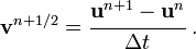
The finite element system of equations is

\mathbf{M}~\ddot{\mathbf{u}} = \mathbf{f}_{\text{ext}} - \mathbf{f}_{\text{int}} = \mathbf{f} ~.

Let's assume that the mass matrix is diagonal. Let us also assume that we would like to solve this problem using an explicit method that uses central differencing.

Let the time step size be $\Delta t$ . Let us also assume that the time step is constant. Then, at time step $n$ , the time is $t_n = n\Delta t$ .

Let

\mathbf{u}_n = \mathbf{u}(t_n) ~.

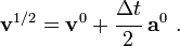
Let us take a half step to compute the velocity at the middle of the timestep. Then,

\mathbf{v}^{n+1/2} = \cfrac{\mathbf{u}^{n+1} - \mathbf{u}^n}{\Delta t} ~.

We will use this half-step velocity to compute the acceleration

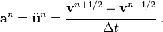
\mathbf{a}^n = \ddot{\mathbf{u}}^n = \cfrac{\mathbf{v}^{n+1/2} - \mathbf{v}^{n-1/2}}{\Delta t} ~.

Now,

\ddot{\mathbf{u}}^n = \mathbf{M}^{-1}~\mathbf{f}^n ~.

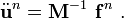
Therefore,

\mathbf{M}^{-1}~\mathbf{f}^n =\cfrac{\mathbf{v}^{n+1/2} - \mathbf{v}^{n-1/2}}{\Delta t} \qquad \implies \qquad \mathbf{v}^{n+1/2} = \mathbf{v}^{n-1/2} + \Delta t~\mathbf{M}^{-1}~\mathbf{f}^n ~.

Algorithm

Initialize:
1. Set $t = 0$ and $n = 0$ .
2. Set the initial velocities ( $\mathbf{v}^0$ ) at the nodes.
3. Set the initial accelerations ( $\mathbf{a}^0$ ) at the nodes.
4. Set the initial stresses ( $\sigma^0$ ) at the element Gauss points.
5. Compute the lumped mass $\mathbf{M}$ at the nodes.
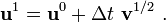
Set the displacements and velocities at the first time step:
1. Displacement: $\mathbf{u}^0 = 0 ~.$
2. Velocity: $\mathbf{v}^{1/2} = \mathbf{v}^0 + \cfrac{\Delta t}{2}~\mathbf{a}^0 ~.$
Apply essential BCs: $[\mathbf{v}^{1/2}]_{\Gamma_v} = \bar{\mathbf{v}}(\mathbf{x}, \Delta t/2) ~.$
Update the nodal displacements: $\mathbf{u}^1 = \mathbf{u}^0 + \Delta t~\mathbf{v}^{1/2} ~.$
Set $n=1$ and $t = \Delta t$ .
Loop through the following steps until $t = t_{\text{max}}$ .
For each element (at the Gauss points):
1. Compute the strain measure: $\varepsilon^n = u_{,X} ~~\text{or}~~ D^n = v_{,x} ~.$
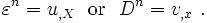
2. Compute the stress: $P = E^{PF}~\varepsilon^n ~~\text{or}~~ \dot{\sigma} = E^{\sigma D}~D^n ~.$
For each node:
1. Compute the internal force $(f_i^n)_{\text{int}}$ .
2. Compute the external force $(f_i^n)_{\text{ext}}$ .
3. Compute the total force $f_i^n$ .
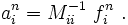
4. Compute the acceleration $a_i^n$ : $a_i^n = M_{ii}^{-1}~f_i^n ~.$
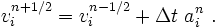
5. Update the velocity $v_i^{n+1/2}$ . $v_i^{n+1/2} = v_i^{n-1/2} + \Delta t~a_i^n ~.$
6. Apply the essential boundary conditions.
7. Update the displacement $u_i^{n+1}$ . $u_i^{n+1} = u_i^n + \Delta t~v_i^{n+1/2}~.$
Update the counters: $n = n+1$ , $t = t + \Delta t$ .

Stability of the Explicit Algorithm

If the time step $\Delta t$ is too large, the algorithm may not be stable and may give unreasonable results. To provide a check on the time step size, we use the CFL (Courant-Friedrichs-Lewy) condition to determine $\Delta t$ . This condition (in 1-D) states that

{ \Delta t_{\text{crit}} = \cfrac{l_0}{c_0} }

where $l_0$ is the initial length of the element, and $c_0$ is speed of sound in the material (wavespeed) given by

{ c_0 = \cfrac{E^{PF}}{\rho_0} ~. }

This article is issued from Wikiversity - version of the Wednesday, August 15, 2007. The text is available under the Creative Commons Attribution/Share Alike but additional terms may apply for the media files.