Nonlinear finite elements/Solution of heat equation
< Nonlinear finite elementsFinite element solution for the Heat equation
Let us now try to create a finite element approximation for the variational initial boundary value problem for the heat equation . This problem can be stated as
![{
\begin{align}
& \mathsf{ Variational~ IBVP ~for~ the~ Heat~ Equation}\\
& \\
\text{Find a function} & ~T(t) \in \mathcal{S}_t, t \in [0,\tau]
~\text{such that for all}~ w \in \mathcal{V}\\
& \\
& \int_{\Omega} \left(\rho~C_v~\frac{\partial T}{\partial t}\right)~w~dV +
\int_{\Omega} (\boldsymbol{\nabla} w)\bullet(\boldsymbol{\kappa}\bullet\boldsymbol{\nabla} T)~dV=
\int_{\Omega} s~w~dV -
\int_{\Gamma_q} w~\overline{q}~dA \\
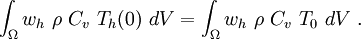
& \int_{\Omega} w~\rho~C_v~T(0)~dV =
\int_{\Omega} w~\rho~C_v~T_0~dV ~.
\end{align}
}](../I/m/0929163e60bb329ee058b1bb13e7d524.png)
Let  be a finite dimensional approximation to
  and let
 be a finite dimensional approximation to
  . Let the
weighting functions
. Let the
weighting functions  be such that
  on
on  .
Similarly, any other function
.
Similarly, any other function  also goes to zero on the
boundary .
also goes to zero on the
boundary .
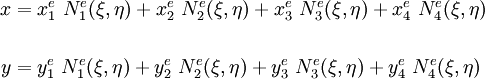
Assume that the trial solutions  can be represented as

The additional quantity  results in the satisfaction of the
boundary condition
results in the satisfaction of the
boundary condition  on .
on .
If we substitute these quantities into the variational initial boundary value problem, we get the Galerkin formulation. The steps in this process are shown below.
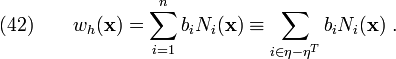
Approximate IBVP
The approximate form of the variational IBVP is

Replacing  with
with  we get

After expanding and rearranging terms, we get
In compact notation

Similarly, the initial condition can be written as
Substituting for and expanding out terms, we have

In compact form,

Therefore the approximate form of the variational BVP can be written as
![\text{(40)} \qquad
{
\begin{align}
& \mathsf{ Approximate~ Variational~ IBVP~ for~ the~ Heat~ Equation}\\
& \\
\text{Find a function} & ~T_h(t) = v_h + \overline{T}_h \in \mathcal{S}_h,
t \in [0,\tau] ~\text{such that for all}~ w_h \in \mathcal{V}_h\\
& \\
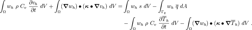
\int_{\Omega} w_h~\rho~C_v~\frac{\partial v_h}{\partial t}~dV & +
\int_{\Omega} (\boldsymbol{\nabla} w_h)\bullet(\boldsymbol{\kappa}\bullet\boldsymbol{\nabla} v_h)~dV
= \int_{\Omega} w_h~s~dV - \int_{\Gamma_q} w_h~\overline{q}~dA \\
& - \int_{\Omega} w_h~\rho~C_v~\frac{\partial \overline{T}_h}{\partial t}~dV
-\int_{\Omega}
(\boldsymbol{\nabla} w_h)\bullet(\boldsymbol{\kappa}\bullet\boldsymbol{\nabla} \overline{T}_h)~dV ~. \\
\int_{\Omega} w_h~\rho~C_v~v_h(0)~dV & =
\int_{\Omega} w_h~\rho~C_v~T_0~dV-
\int_{\Omega} w_h~\rho~C_v~\overline{T}_h(0)~dV ~.
\end{align}
}](../I/m/47bab63143a51bb00d82bba15d813a2c.png)
Note that the derivatives with respect to time are still continuous in this approximate variational BVP.
Finite element approximation
We now discretize our domain into elements  where
where  and
and  is the total number of elements. Nodes may exist anywhere within
the element domains. But the most common locations are at the element
vertices and along the interelement boundaries.
is the total number of elements. Nodes may exist anywhere within
the element domains. But the most common locations are at the element
vertices and along the interelement boundaries.
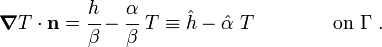
Let the set of global node numbers be
Let the set nodes at which a temperature (essential BC) is prescribed be

Then the set of nodes at which a temperature is to be determined is the complement

Let  be the number of nodes in
  . Then the number of
equations to be solved is also . See Figure 1
to get an idea about what these sets of nodes refer to.
. Then the number of
equations to be solved is also . See Figure 1
to get an idea about what these sets of nodes refer to.
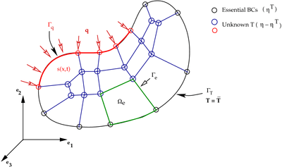 Figure 1. FEM discretization for the heat conduction problem. |
As we have seen before, a typical weighting function
is assumed to have the form
Note that only if  for every
  . On
the other hand for every node in
. On
the other hand for every node in  .
.
Similarly, a typical trial solution can be written as
where  is the unknown temperature at node
  at time
  .
.
We also often represent the approximate form of the essential BCs in a similar way, i.e.,
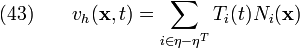
Substitute equations (42), (43), and (44) into the first of equations (40). You will get
![\begin{align}
\int_{\Omega} \left(\sum_j b_j N_j\right)~
& \rho~C_v~\left(\sum_i \frac{\partial T_i}{\partial t} N_i\right)~dV +
\int_{\Omega} \left(\sum_j b_j \boldsymbol{\nabla} N_j\right)\bullet
\left[\sum_i T_i
\left(\boldsymbol{\kappa}\bullet\boldsymbol{\nabla} N_i\right)\right]~dV
=\\
& \int_{\Omega} \left(\sum_j b_j N_j\right)~s~dV -
\int_{\Gamma_q} \left(\sum_j b_j N_j\right)~\overline{q}~dA\\
& - \int_{\Omega} \left(\sum_j b_j N_j\right)~
\rho~C_v~\left(\sum_k \frac{\partial \overline{T}_k}{\partial t} N_k\right)~dV \\
& - \int_{\Omega}
\left(\sum_j b_j \boldsymbol{\nabla} N_j\right)\bullet
\left[\sum_k \overline{T}_k
\left(\boldsymbol{\kappa}\bullet\boldsymbol{\nabla} N_k\right)\right]~dV
, \qquad i,j \in \eta - \eta^T, \quad k \in \eta^T~.
\end{align}](../I/m/06c9a216f666cff513a235443bae7460.png)
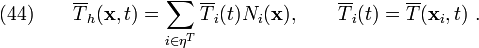
Assuming that  does not change with time, we can take the
constants and time-dependent parameters outside the integrals to get
does not change with time, we can take the
constants and time-dependent parameters outside the integrals to get
![\begin{align}
\sum_j b_j & \left[
\sum_i \frac{\partial T_i}{\partial t}\left(\int_{\Omega}\rho~C_v~N_i~N_j~dV\right) +
\sum_i T_i\left(\int_{\Omega}\boldsymbol{\nabla} N_j \bullet
(\boldsymbol{\kappa}\bullet\boldsymbol{\nabla} N_i)~dV
\right)\right] =\\
& \sum_j b_j \left[
\int_{\Omega} N_j~s~dV -
\int_{\Gamma_q} N_j~\overline{q}~dA -
\sum_k \frac{\partial \overline{T}_k}{\partial t}
\left(\int_{\Omega} \rho~C_v~N_j~N_k~dV\right)\right. \\
& - \left.\sum_k \overline{T}_k
\left(\int_{\Omega} \boldsymbol{\nabla} N_j\bullet(\boldsymbol{\kappa}\bullet\boldsymbol{\nabla} N_k)~dV
\right)\right]
, \qquad i,j \in \eta - \eta^T, \quad k \in \eta^T~.
\end{align}](../I/m/c8050fccc5d86b7cae2ac99e3d0db27c.png)
Using the usual argument about the arbitrary nature of  , we get
In compact notation,

where  , and
, and  .
.
Let us rename parts of the above equation as follows:
Then we get

In matrix form,
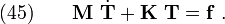
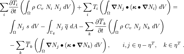
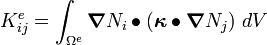
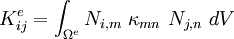
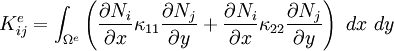
As before, we can break up the global matrices into sums over elements. Thus,
where
![\begin{align}
M^e_{ij} & = \int_{\Omega^e} \rho~C_v~N_i~N_j~dV~,\\
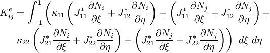
K^e_{ij} & =
\int_{\Omega^e}\boldsymbol{\nabla} N_i\bullet(\boldsymbol{\kappa}\bullet\boldsymbol{\nabla} N_j)~dV
\equiv \int_{\Omega^e} \mathbf{B}^T_i~\mathbf{D}~\mathbf{B}_j~dV ~, \\
f^e_j & = \int_{\Omega^e} N_j~s~dV -
\int_{\Gamma^e_q} N_j~\overline{q}~dA -
\sum_{k=1}^{n^e} \left[
M^e_{jk} \dot{\overline{T}}_k -
K^e_{jk} \overline{T}_k \right]
\end{align}](../I/m/3d7c5df50e5db02fa3d0521194ce9fd2.png)
and  is the number of nodes in an element.
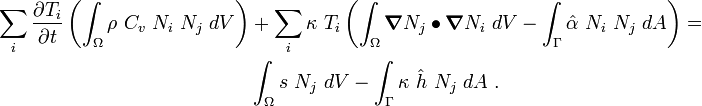
We can do the same for the initial conditions. However, a more common
approach is to specify the values of  directly at the nodes
instead of going through an assembly process.
directly at the nodes
instead of going through an assembly process.
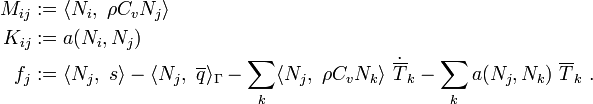
Computing  ,
,  ,
, 
The finite element system of equations at time :
![\begin{align}
M^e_{ij} & = \int_{\Omega^e} \rho~C_v~N_i~N_j~dV~,\\
K^e_{ij} & =
\int_{\Omega^e}\boldsymbol{\nabla} N_i\bullet({\boldsymbol{\kappa}\bullet{\boldsymbol{\nabla} N_j})}~dV
\equiv \int_{\Omega^e} \mathbf{B}^T_i~\mathbf{D}~\mathbf{B}_j~dV ~, \\
f^e_j & = \int_{\Omega^e} N_j~s~dV -
\int_{\Gamma^e_q} N_j~\overline{q}~dA -
\sum_{k=1}^{n^e} \left[
M^e_{jk} \dot{\overline{T}}_k -
K^e_{jk} \overline{T}_k \right]
\end{align}](../I/m/e4cbbf369bdfac620f0dd3f4abb1b24e.png)
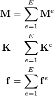
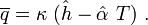
Isoparametric Map
 Isoparametric map. |
Coordinate Transformation
Integrating Stiffness Matrix
Stiffness matrix terms:
Index notation:
Expanded out (in 2D) (assume  ):
):
Transformation
Chain Rule:
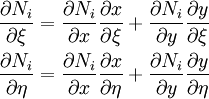
Matrix notation:
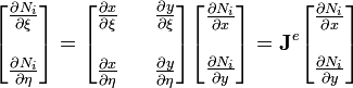
Inverse Transformation
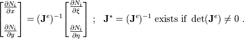
with
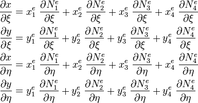
Returning to the integration of the stiffness matrix terms:
In parent element coordinates:
Gaussian Quadrature
Gaussian Quadrature Example
Find the constants Co, C1, and X so that the quadrature formula
This has the highest possible degree of precision.
Solution.
Since there are three unknowns, Co, C1 and X1, we will expect the formula to be exact for
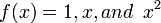
Thus

Equation 2 and 3 will yield.
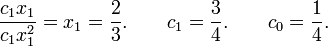
Hence
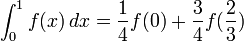
Now,
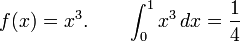
And
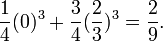
Thus the degree of the precision is 2
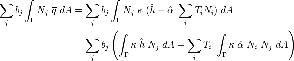
Robin boundary conditions
A similar approach can be used when w:Robin boundary conditions are needed to be applied. Let us assume that the Robin boundary conditions take the form

Recall from the previous section that the boundary term in the weak form of the heat equation is

where
 .
.
Let us assume, for simplicity, that the material is isotropic. In that case  becomes a scalar quantity
  and we can write
Now, we can write the Robin boundary condition as
Using this expression we can get of the flux term in  to get
Then the boundary term takes the form
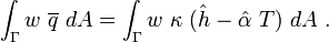
If we ignore the contributions to the trial function from the Dirichlet boundary conditions we can write
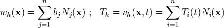
Plugging these expressions into the boundary term leads to
Now recall that spatially discretized equation for transient heat conduction can be expressed as (in simplified form; after getting rid of contributions due to Dirichlet boundary conditions and with a scalar )
![\begin{align}
\sum_j b_j & \left[
\sum_i \frac{\partial T_i}{\partial t}\left(\int_{\Omega}\rho~C_v~N_i~N_j~dV\right) +
\sum_i \kappa~T_i\left(\int_{\Omega}\boldsymbol{\nabla} N_j \bullet
\boldsymbol{\nabla} N_i~dV
\right)\right] =\\
& \sum_j b_j \left[
\int_{\Omega} N_j~s~dV -
\int_{\Gamma} N_j~\overline{q}~dA\right]
\end{align}](../I/m/718324c7d77d6d99777a2c71ede83232.png)
Substituting the last term on the right hand side with the new expression for the boundary term, we have
![\begin{align}
\sum_j b_j & \left[
\sum_i \frac{\partial T_i}{\partial t}\left(\int_{\Omega}\rho~C_v~N_i~N_j~dV\right) +
\sum_i \kappa~T_i\left(\int_{\Omega}\boldsymbol{\nabla} N_j \bullet
\boldsymbol{\nabla} N_i~dV
\right)\right] =\\
& \sum_j b_j \left[
\int_{\Omega} N_j~s~dV - \kappa~\int_{\Gamma} \hat{h}~N_j~dA +
\sum_i \kappa~T_i~\int_{\Gamma} \hat{\alpha}~N_i~N_j~dA
\right]
\end{align}](../I/m/bfa404020dc0cf0dbe109560dc2ee544.png)
Invoking the arbitrariness of and rearranging, we get
Define
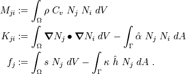
Then the finite element system of equations is
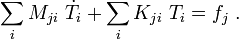
or, in matrix form
Note that the matrix and the vector are different from the case where there are no Robin boundary conditions. The boundary terms in the discretized system of equations can be computed in the usual manner and will add terms to the diagonal of the matrix.