Nonlinear finite elements/Solution of Poisson equation

Construction of Approximate Solutions

If we know that the problem is well-posed but does not have a closed form solution, we can go ahead and try to get an approximate solution. The finite element method is one way of getting at approximate solutions (among many other numerical methods).

The finite element method starts off with the variational form (or the weak form) of the BVP. The method is a special case of a class of methods called Galerkin methods.

Finite element solution for the Poisson equation

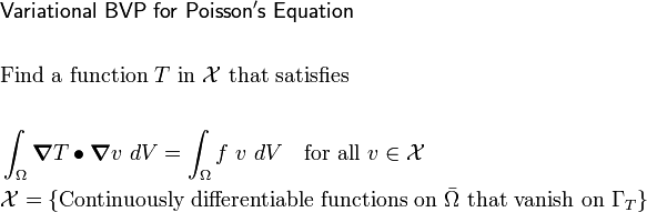
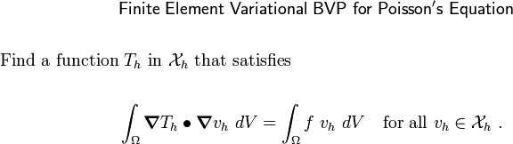
Recall the variational boundary value problem for the Poisson equation:

 ${ \begin{align} &\mathsf{ Variational~ BVP ~for ~Poisson's~ Equation}\\ & \\ &\text{Find a function}~T~\text{in}~\mathcal{X}~\text{that satisfies}\\ & \\ & \int_{\Omega} \boldsymbol{\nabla} T\bullet\boldsymbol{\nabla} v~dV = \int_{\Omega} f~v~dV \quad \text{for all}~v \in \mathcal{X} & \\ &\mathcal{X} = \{\text{Continuously differentiable functions on}~\bar{\Omega}~ \text{that vanish on}~\Gamma_T\} \end{align} }$

The space $\mathcal{X}$ is continuous and an infinite number of functions could be chosen from this space of functions. In the finite element method, we choose a trial function from the space of approximate solutions $\mathcal{X}_h$ where $\mathcal{X}_h \subset \mathcal{X}$ . A defining feature of these approximate trial solutions is that they are associated with a mesh or discretization of the domain $\Omega$ . These functions also have the feature that they are finite dimensional with each dimension being associated with a node on the mesh.

Assume that we are given $\mathcal{X}_h$ . Let us choose a weighting function $v_h \in \mathcal{X}_h$ that satisfies $v_h = 0$ on $\Gamma_T$ . We can choose another function $T_h \in \mathcal{X}_h$ as our trial solution. Since the boundary condition on $\Gamma_T$ is $T = 0$ , both $v_h$ and $T_h$ can have the same form. In the next section, we will look at the general form of the heat equation where $T \ne 0$ on the boundary.

In finite element methods we choose trial solutions $T_h$ of the form

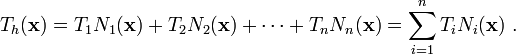
T_h(\mathbf{x}) = T_1 N_1(\mathbf{x}) + T_2 N_2(\mathbf{x}) + \dots + T_n N_n(\mathbf{x}) = \sum_{i=1}^n T_i N_i(\mathbf{x}) ~.

where $T_1$ , $T_2$ , $\dots$ , $T_n$ are nodal temperatures which are constant on $\bar{\Omega}$ . The functions $N_1, N_2, \dots, N_n$ form a basis that spans the subspace $\mathcal{X}_h$ and are known as basis functions or shape functions. Note that $n$ is the total number of nodes minus the number of nodes on $\Gamma_T$ where $T$ is specified.

Since the functions $v_h$ come from the same space of functions, we can represent them as

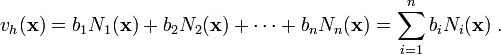
v_h(\mathbf{x}) = b_1 N_1(\mathbf{x}) + b_2 N_2(\mathbf{x}) + \dots + b_n N_n(\mathbf{x}) = \sum_{i=1}^n b_i N_i(\mathbf{x}) ~.

where $b_1$ , $b_2$ , $\dots$ , $b_n$ are arbitrary constant on $\bar{\Omega}$ with the restriction that $v_h = 0$ on $\Gamma_T$ .

If we plug in these finite dimensional forms of $v$ and $T$ into the variational BVP, we get an approximate form of the variational BVP which can be stated as:

 ${ \begin{align} &\mathsf{Finite~ Element ~Variational~ BVP~ for~ Poisson's~ Equation}\\ & \\ \text{Find a function}& ~T_h~\text{in}~\mathcal{X}_h~\text{that satisfies}\\ & \\ & \int_{\Omega} \boldsymbol{\nabla} T_h\bullet\boldsymbol{\nabla} v_h~dV = \int_{\Omega} f~v_h~dV \quad \text{for all}~v_h \in \mathcal{X}_h ~. \end{align} }$

After substituting the expressions for $v_h$ and $T_h$ in the variational BVP we get

\begin{align} 0 & = \int_{\Omega} \boldsymbol{\nabla} T_h\bullet\boldsymbol{\nabla} v_h~dV - \int_{\Omega} f~v_h~dV \\ & = \int_{\Omega} \boldsymbol{\nabla} (T_1 N_1+\dots+T_n N_n)\bullet \boldsymbol{\nabla} (b_1 N_1+\dots+b_n N_n)~dV - \int_{\Omega} f~(b_1 N_1+\dots+b_n N_n)~dV \\ & = \int_{\Omega} (T_1\boldsymbol{\nabla} N_1+\dots+T_n\boldsymbol{\nabla} N_n)\bullet (b_1\boldsymbol{\nabla} N_1+\dots+b_n\boldsymbol{\nabla} N_n)~dV - \int_{\Omega} f~(b_1 N_1+\dots+b_n N_n)~dV \\ & = \sum_{i,j=1}^n K_{ij} T_i b_j - \sum_{j=1}^n f_j b_j \\ & = \sum_{j=1}^n b_j \left[\sum_{i=1}^n K_{ij} T_i - f_j\right] \\ \end{align}

where,

{ K_{ij} = \int_{\Omega} \boldsymbol{\nabla} N_i\bullet\boldsymbol{\nabla} N_j~dV ~~~~\text{and}~~~ f_{j} = \int_{\Omega} f N_j~dV~. }

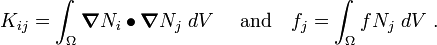
In matrix form, we have

\text{(38)} \qquad \mathbf{b}^{T} \left[\mathbf{K} \mathbf{T} - \mathbf{f}\right] = \mathbf{0}

where $\mathbf{b}^T = [b_1, b_2, \dots, b_n]$ , $\mathbf{K}$ is a $n \times n$ symmetric matrix, $\mathbf{T} = [T_1, T_2, \dots, T_n]$ is a $n \times 1$ vector, and $\mathbf{f}$ is a $n \times 1$ vector.

Since $\mathbf{b}$ can be arbitrary, equation (38) can be further simplified to the form

\text{(39)} \qquad { \mathbf{K} \mathbf{T} = \mathbf{f} }

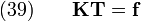
This system of equations has a solution since $\mathbf{K}$ is positive-definite and therefore has an inverse. Once the $T_i$ s are known, the approximate solution can be found using

T_h(\mathbf{x}) = T_1 N_1(\mathbf{x}) + T_1 N_2(\mathbf{x}) + \dots + T_n N_n(\mathbf{x}) ~.

The functions $N_1, \dots, N_n$ have special forms in the finite element method that have the property that the quality of the approximation improves with an increase in the dimension $n$ of the basis.

This article is issued from Wikiversity - version of the Wednesday, April 23, 2008. The text is available under the Creative Commons Attribution/Share Alike but additional terms may apply for the media files.