Nonlinear finite elements/Rate form of hyperelastic laws
< Nonlinear finite elementsRate equations
Let us now derive rate equations for a hyperelastic material.
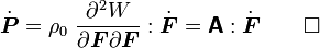
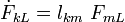
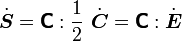
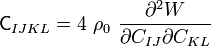
First elasticity tensor
We start off with the relation
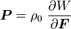
Then the material time derivative of  is given by
|
First elasticity tensor |
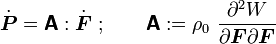
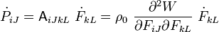
where the fourth order tensor  is call the first elasticity tensor. This tensor has major symmetries but not minor symmetries. In
index notation with respect to an orthonormal basis
is call the first elasticity tensor. This tensor has major symmetries but not minor symmetries. In
index notation with respect to an orthonormal basis
Proof:
We have
Using the product rule, we have
Therefore,


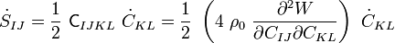
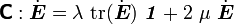
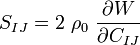
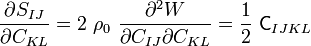
Second elasticity tensor
Similarly, if we start off with the relation
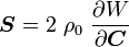
the material time derivative of  can be expressed as
|
Second elasticity tensor |
where the fourth order tensor  is called the material elasticity tensor or the second elasticity tensor. Since this tensor relates symmetric second order tensors it has minor symmetries. It also has major symmetries because the two partial derivatives are with the same quantity and an interchange does not change
things. In index notation with respect to an orthonormal basis
is called the material elasticity tensor or the second elasticity tensor. Since this tensor relates symmetric second order tensors it has minor symmetries. It also has major symmetries because the two partial derivatives are with the same quantity and an interchange does not change
things. In index notation with respect to an orthonormal basis
Proof:
We have
Again using the product rule, we have
Therefore,


|
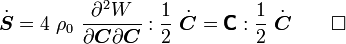
The first and second elasticity tensors are related by |

Proof:
Recall that the first and second Piola-Kirchhoff stresses are related by
Taking the material time derivative of both sides gives
Using the expression for
above, we get
Now
Therefore,
Now
That means
which gives us
In index notation,
Therefore,

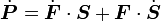

![\dot{\boldsymbol{P}} = \dot{\boldsymbol{F}}\cdot\boldsymbol{S} + \frac{1}{2}~\boldsymbol{F}\cdot[\boldsymbol{\mathsf{C}}:(
\dot{\boldsymbol{F}^T}\cdot\boldsymbol{F} + \boldsymbol{F}^T\cdot\dot{\boldsymbol{F}})]](../I/m/b6c67e049782168223f99034ce6d58b7.png)

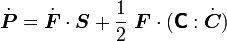
![\dot{\boldsymbol{P}} = \dot{\boldsymbol{F}}\cdot\boldsymbol{S} + \boldsymbol{F}\cdot[\boldsymbol{\mathsf{C}}:(\boldsymbol{F}^T\cdot\dot{\boldsymbol{F}})]](../I/m/258a766147a375e41850de1873319171.png)
![\begin{align}
\dot{P}_{iJ} & = \dot{F}_{iL}~S_{LJ} + F_{iN}~[\mathsf{C}_{NJML}~F_{kM}~\dot{F}_{kL}]\\
& = S_{LJ}~\delta_{ik}\dot{F}_{kL}+\mathsf{C}_{NJML}~F_{iN}~F_{kM}~\dot{F}_{kL}\\
& = (\delta_{ik}~S_{JL} + F_{iN}~\mathsf{C}_{NJML}~F_{kM})~\dot{F}_{kL}
& = \mathsf{A}_{iJkL}~\dot{F}_{kL}
\end{align}](../I/m/ee3a0db9a312b99c0d4dbdabc348621f.png)

Fourth elasticity tensor
Now we will compute the spatial elasticity tensor for the rate constitutive equation for a hyperelastic material. This tensor relates an objective rate of stress (Cauchy or Kirchhoff) to the rate of deformation tensor. We can show that
|
Fourth elasticity tensor for the Kirchhoff stress where |
![{
\mathcal{L}_\varphi[\boldsymbol{\tau}] = \boldsymbol{\mathsf{c}}:\boldsymbol{d} \equiv
\boldsymbol{\mathsf{c}}_{\tau}:\boldsymbol{d}
}](../I/m/14214d855dfa0f1fab96fac21ac00b17.png)

The fourth order tensor  is called the spatial elasticity tensor or the fourth elasticity tensor. Clearly,
  cannot be derived from the store energy function
  because of the dependence on the deformation gradient.
Proof:
Recall that the Lie derivative of the Kirchhoff stress is defined as
We have found that
We also know from Continuum_mechanics/Time_derivatives_and_rates#Time_derivative_of_strain that
where
is the spatial rate of deformation tensor. Therefore,
In index notation,
or,
where
![\mathcal{L}_\varphi[\boldsymbol{\tau}] = \overset{\circ}{\boldsymbol{\tau}} = \boldsymbol{F}\cdot\dot{\boldsymbol{S}}\cdot\boldsymbol{F}^T](../I/m/0a24196ff7c7d046c3cacb82181999a5.png)
![\mathcal{L}_\varphi[\boldsymbol{\tau}] = \boldsymbol{F}\cdot[\boldsymbol{\mathsf{C}}:(\boldsymbol{F}^T\cdot\boldsymbol{d}\cdot\boldsymbol{F})]\cdot\boldsymbol{F}^T](../I/m/3efbb318043043d5644e67f99f043ee8.png)
![(\mathcal{L}_\varphi[\boldsymbol{\tau}])_{ij} = F_{iK}~\mathsf{C}_{KLMN}~F_{kM}~d_{kl}~F_{lN}~F_{jL}
= F_{iK}~F_{jL}~F_{kM}~F_{lN}~\mathsf{C}_{KLMN}~d_{kl}
= \mathsf{c}_{ijkl}~d_{kl}](../I/m/2bd99883f6974cf08e751b62be4ee402.png)
![\mathcal{L}_\varphi[\boldsymbol{\tau}] = \boldsymbol{\mathsf{c}}:\boldsymbol{d}](../I/m/7f458702d6d9bfb3fd11e31734ab9ff5.png)

Alternatively, we may define in terms of the Cauchy stress  , in which
case the constitutive relation is written as
, in which
case the constitutive relation is written as
|
Fourth elasticity tensor for the Cauchy stress where |
![{
\mathcal{L}_\varphi[\boldsymbol{\sigma}] = \boldsymbol{\mathsf{c}}:\boldsymbol{d} = J^{-1}~\boldsymbol{\mathsf{c}}_{\tau}:\boldsymbol{d}
}](../I/m/80fd241e2f8d0da56f50b464ea6a8429.png)

The proof of this relation between the spatial and material elasticity tensors is very similar to that for the rate of Kirchhoff stress. Many authors define this quantity as the spatial elasticity
tensor. Note the factor of  . This form of the spatial elasticity tensor is crucial for some of the calculations that follow.
|
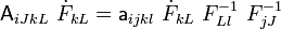
The first and fourth elasticity tensors are related by In the above equation Instead, if we use the Cauchy stress and the spatial elasticity tensor |
![{
\mathsf{A}_{iJkL} = F_{Jj}^{-1}[\mathsf{c}_{ijkl} + \tau_{ij}~\delta_{kl}]~F_{Ll}^{-1}
}](../I/m/7b300ddb1c1ef5d687144d30aedd205e.png)
![{
\mathsf{A}_{iJkL} = J~F_{Jj}^{-1}[\mathsf{c}_{ijkl} + \sigma_{ij}~\delta_{kl}]~F_{Ll}^{-1}
}](../I/m/ca215c36d79429fb85abab2568c9869d.png)
Proof:
Recall that
Therefore,
Also recall that
Therefore, using index notation,
Now,
In index notation
Using this we get
or,
Now,
Therefore,
Also,
So we have
Note:
The fourth order tensor
which depends on the symmetry of
is called the third elasticity tensor, i.e.,
Therefore, the relation between the first and third elasticity tensors is
or,
In index notation
Therefore,


![\boldsymbol{\mathsf{A}}:\dot{\boldsymbol{F}} = [\boldsymbol{\mathsf{a}}:(\dot{\boldsymbol{F}}\cdot\boldsymbol{F}^{-1})]\cdot\boldsymbol{F}^{-T}](../I/m/2cabcadd88a7a0452fe41abac716fd91.png)

An isotropic spatial elasticity tensor?
An isotropic spatial elasticity tensor cannot be derived from a stored energy function if the constitutive relation is of the form
where

Since a significant number of finite element codes use such a constitutive equation, (also called the equation of a hypoelastic material of grade 0) it is worth examining why such a model is incompatible with elasticity.
Start with a constant and isotropic material elasticity tensor
Let us start of with an isotropic elastic material model in the reference configuration. The simplest such model is the St. Venant-Kirchhoff hyperelastic model
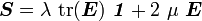
where is the second Piola-Kirchhoff stress,  is the Lagrangian Green strain,
and
is the Lagrangian Green strain,
and  are material constants. We can show that this equation can be
derived from a stored energy function.
are material constants. We can show that this equation can be
derived from a stored energy function.
Taking the material time derivative of this equation, we get
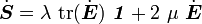
Now,
where is the second (material) elasticity tensor.
Therefore,
which implies that

In index notation,

Now, from the relations between the second elasticity tensor and the fourth (spatial) elasticity tensor, we have

Therefore, in this case,
![\mathsf{c}_{ijkl} = F_{iI}~F_{jJ}~F_{kK}~F_{lL}~\left[
\lambda~\delta_{IJ}~\delta_{KL} + \mu~(\delta_{IK}~\delta_{JL} +
\delta_{JK}~\delta_{IL})\right]](../I/m/fcb22c48b5f56263130e0948162d51fc.png)
or,

where  . So we see that the spatial elasticity tensor
cannot be a constant tensor unless
. So we see that the spatial elasticity tensor
cannot be a constant tensor unless  .
.
Alternatively, if we define

we get

Start with a constant and isotropic spatial elasticity tensor
Let us now look at the situation where we start off with a constant and isotropic spatial elasticity tensor, i.e.,
In index notation,

Since
multiplying both sides by  we have,

Therefore, substituting in the expression for a constant and isotropic , we
have
![\mathsf{C}_{ABCD} =
F^{-1}_{Ai}~F^{-1}_{Bj}~F^{-1}_{Ck}~F^{-1}_{Dl}~\left[
\lambda~\delta_{ij}~\delta_{kl} + \mu(
\delta_{ik}~\delta_{jl} + \delta_{jk}~\delta_{il})\right]](../I/m/9c3059ae22c060a5917de323cb3ccaa7.png)
or,

or,

Since  which gives us
  , we
can write
, we
can write

Alternatively, if we define
we get

and therefore,

Hypoelastic material of grade 0
A hypoelastic material of grade zero is one for which the stress-strain relation in rate form can be expressed as
![\mathcal{L}_{\varphi}[\boldsymbol{\sigma}] = \boldsymbol{\mathsf{c}}:\boldsymbol{d}](../I/m/3ea80e934bad9b72563954d30915c7f1.png)
where is constant. When the material is isotropic we have
We want to show that hypoelastic material models of grade 0 cannot be derived from a stored energy function. To do that, recall that
and
For a material elasticity tensor to be derivable from a stored energy function
it has to satisfy the Bernstein integrability conditions. We have
Also, due to the interchangeability of derivatives,
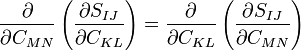
Therefore,

These integrability conditions have to be satisfied by any material elasticity tensor.
At this stage we will use the relation

If we plug this into the integrability condition we will see that

If we multiply both sides by  we are left with

This is an unphysical situation and hence shows that a hypoelastic material of
grade zero requires that  for it to be derivable from a stored
energy function.
for it to be derivable from a stored
energy function.
Proof:
Let us simplify the notation by writing
. Then,
Then,
and
As this stage we use the identities (see Nonlinear finite elements/Kinematics#Some_useful_results for proofs)
and
Therefore we have
and
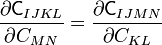
Equating the two, we see that the terms that cancel out are
and
Therefore,
implies that
or,
In other words,
Now, if we multiply both sides by
we get
or,
Next, multiplying both sides by
gives
or,
Finally, multiplying both sides by
gives
Therefore,

![\begin{align}
\frac{\partial \mathsf{C}_{IJKL}}{\partial C_{MN}} = &
\lambda~\frac{\partial J}{\partial C_{MN}}~A_{IJ}~A_{KL} + \\
& J~\lambda~\left[\frac{\partial A_{IJ}}{\partial C_{MN}}~A_{KL} +
A_{IJ}~\frac{\partial A_{KL}}{\partial C_{MN}}\right] + \\
& \mu~\frac{\partial J}{\partial C_{MN}}~(A_{IK}~A_{JL} + A_{JK}~A_{IL}) + \\
& J~\mu~\left[\frac{\partial A_{IK}}{\partial C_{MN}}~A_{JL} +
A_{IK}~\frac{\partial A_{JL}}{\partial C_{MN}} +
\frac{\partial A_{JK}}{\partial C_{MN}}~A_{IL} +
A_{JK}~\frac{\partial A_{IL}}{\partial C_{MN}}\right]
\end{align}](../I/m/29b32b00b5d2ca166e849bc5a9671956.png)
![\begin{align}
\frac{\partial \mathsf{C}_{IJMN}}{\partial C_{KL}} = &
\lambda~\frac{\partial J}{\partial C_{KL}}~A_{IJ}~A_{MN} + \\
& J~\lambda~\left[\frac{\partial A_{IJ}}{\partial C_{KL}}~A_{MN} +
A_{IJ}~\frac{\partial A_{MN}}{\partial C_{KL}}\right] + \\
& \mu~\frac{\partial J}{\partial C_{KL}}~(A_{IM}~A_{JN} + A_{JM}~A_{IN}) + \\
& J~\mu~\left[\frac{\partial A_{IM}}{\partial C_{KL}}~A_{JN} +
A_{IM}~\frac{\partial A_{JN}}{\partial C_{KL}} +
\frac{\partial A_{JM}}{\partial C_{KL}}~A_{IN} +
A_{JM}~\frac{\partial A_{IN}}{\partial C_{KL}}\right]
\end{align}](../I/m/704ff21dc0fa3bae9ba25d2258e3963c.png)

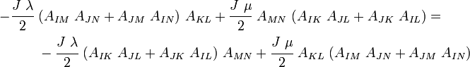
![\begin{align}
\frac{\partial \mathsf{C}_{IJKL}}{\partial C_{MN}} = &
\cfrac{J~\lambda}{2}~A_{MN}~A_{IJ}~A_{KL} - \\
& \cfrac{J~\lambda}{2}~\left[(A_{IM}~A_{JN} + A_{JM}~A_{IN})~A_{KL} +
(A_{KM}~A_{LN} + A_{LM}~A_{KN})~A_{IJ}\right] + \\
& \cfrac{J~\mu}{2}~A_{MN}~(A_{IK}~A_{JL} + A_{JK}~A_{IL}) - \\
& \cfrac{J~\mu}{2}~\left[(A_{IM}~A_{KN}+A_{KM}~A_{IN})~A_{JL} +
(A_{JM}~A_{LN}+A_{LM}~A_{JN})~A_{IK}\right. + \\
& \qquad\quad \left. (A_{JM}~A_{KN}+A_{KM}~A_{JN})~A_{IL} +
(A_{IM}~A_{LN}+A_{LM}~A_{IN})A_{JK}\right]
\end{align}](../I/m/635e4381c1fbe298419aa313e7565040.png)
![\begin{align}
\frac{\partial \mathsf{C}_{IJMN}}{\partial C_{KL}} = &
\cfrac{J~\lambda}{2}~A_{KL}~A_{IJ}~A_{MN} - \\
& \cfrac{J~\lambda}{2}~\left[(A_{IK}~A_{JL}+A_{JK}~A_{IL})~A_{MN} +
(A_{KM}~A_{LN} + A_{LM}~A_{KN})A_{IJ}\right] + \\
& \cfrac{J~\mu}{2}~A_{KL}~(A_{IM}~A_{JN} + A_{JM}~A_{IN}) - \\
& \cfrac{J~\mu}{2}~\left[(A_{IK}~A_{LM}+A_{KM}~A_{IL})~A_{JN} +
(A_{JK}~A_{LN}+A_{JL}~A_{KN})~A_{IM} + \right.\\
& \qquad \qquad \left. (A_{JK}~A_{LM}+A_{JL}~A_{KM})~A_{IN} +
(A_{IK}~A_{LN}+A_{IL}~A_{KN})~A_{JM}\right]
\end{align}](../I/m/48e2cc14f7480d474e6e7d03653db479.png)

![\begin{align}
\cfrac{J~\mu}{2}~& \left[(A_{IM}~A_{KN}+A_{KM}~A_{IN})~A_{JL} +
(A_{JM}~A_{LN}+A_{LM}~A_{JN})~A_{IK}\right. + \\
& \left. (A_{JM}~A_{KN}+A_{KM}~A_{JN})~A_{IL} +
(A_{IM}~A_{LN}+A_{LM}~A_{IN})A_{JK}\right]
\end{align}](../I/m/00a57a74d7dc5b668d2402d9ac0e1d6a.png)