Nonlinear finite elements/Partial differential equations
< Nonlinear finite elementsPartial differential equations (PDEs) are the most common method by which we model physical problems in engineering. Finite element methods are one of many ways of solving PDEs. This handout reviews the basics of PDEs and discusses some of the classes of PDEs in brief. The contents are based on Partial Differential Equations in Mechanics volumes 1 and 2 by A.P.S. Selvadurai and Nonlinear Finite Elements of Continua and Structures by T. Belytschko, W.K. Liu, and B. Moran.
Definition of a PDE
A PDE is a relationship between an unknown function of several variables and its partial derivatives.
Let  be an unknown function. The independent variables are
  ,
,  ,
,  , and
, and  . We usually write
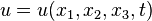
and say that  is the dependent variable.
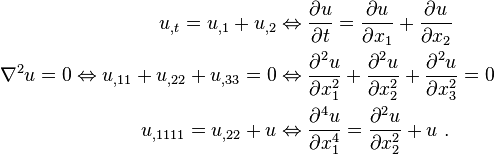
Partial derivatives are denoted by expressions such as

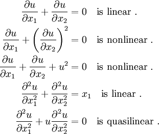
Some examples of partial differential equations are
An example of a system of partial differential equations is

In expanded form this system of equations is
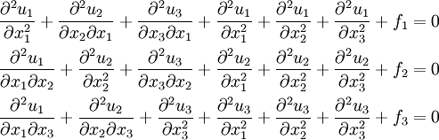
It is often more convenient to write PDEs in vector notation or index notation.
Order of a PDE
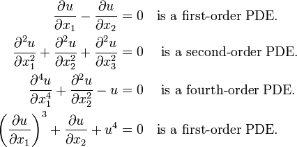
The order of a PDE is determined by the highest derivative in the equation. For example,
Linear and nonlinear PDEs
A linear PDE is one that is of first degree in all of its field variables and partial derivatives. For example,
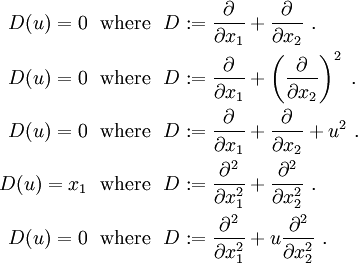
The above equations can also be written in operator notation as
Homogeneous PDEs
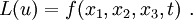
Let  be a linear operator. Then an linear partial differential equation
can be written in the form
be a linear operator. Then an linear partial differential equation
can be written in the form
If 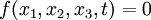 , the PDE is called homogeneous.
Elliptic, Hyperbolic, and Parabolic PDEs
We usually come across three-types of second-order PDEs in mechanics. These are classified as elliptic, hyperbolic, and parabolic.
The equations of elasticity (without inertial terms) are elliptic PDEs. Hyperbolic PDEs describe wave propagation phenomena. The heat conduction equation is an example of a parabolic PDE.
Each type of PDE has certain characteristics that help determine if a particular finite element approach is appropriate to the problem being described by the PDE. Interestingly, just knowing the type of PDE can give us insight into how smooth the solution is, how fast information propagates, and the effect of initial and boundary conditions.
- In hyperbolic PDEs, the smoothness of the solution depends on the smoothness of the initial and boundary conditions. For instance, if there is a jump in the data at the start or at the boundaries, then the jump will propagate as a shock in the solution. If, in addition, the PDE is nonlinear, then shocks may develop even though the initial conditions and the boundary conditions are smooth. In a system modeled with a hyperbolic PDE information travels at a finite speed called the wavespeed. Information is not transmitted until the wave arrives.
- In contrast, the solutions of elliptic PDEs are always smooth, even if the initial and boundary conditions are rough (though there may be singularities at sharp corners). In addition, boundary data at any point affect the solution at all points in the domain.
- Parabolic PDEs are usually time dependent and represent diffusion-like processes. Solutions are smooth in space but may possess singularities. However, information travels at infinite speed in a parabolic system.
Suppose we have a second-order PDE of the form

Then, the PDE is called elliptic if

An example is
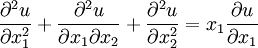
The PDE is called hyperbolic if

An example is
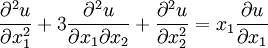
The PDE is called parabolic if

An example is

Solutions to Common PDEs
Partial differential equation appear in several areas of physics and engineering. A firm grasp of how to solve ordinary differential equations is required to solve PDEs. In particular, solutions to the Sturm-Liouville problems should be familiar to anyone attempting to solve PDEs.
Application of PDEs in Physics and Engineering
There are many applications of partial differential equations in physics and engineering. Here are some examples:
- The heat equation
- The diffusion equation
- The wave equation
Resources
The Heat conduction equation of 2-D is elliptic in space and parabolic in time.