Nonlinear finite elements/Overview of balance laws
< Nonlinear finite elementsGoverning equations in the deformed configuration
The governing equations for a continuum (apart from the kinematic relations and the constitutive laws) are
- Balance of mass
- Balance of linear momentum
- Balance of angular momentum
- Balance of energy
- Entropy inequality
Two important results from calculus
There are two important results from calculus that are useful when we use or derive these governing equations. These are
- The Gauss divergence theorem.
- The Reynolds transport theorem
These are useful enough to bear repeating at this point in the context of second order tensors.
The Gauss divergence theorem
The divergence theorem relates volume integrals to surface integrals.
Let  be a body and let
  be its boundary with outward unit normal
 . Let
. Let  be a second order tensor valued function of
  . Then,
if
. Then,
if  is differentiable at least once (i.e.,
  ) then
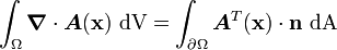
It is often of interest to consider the situation where is not
continuously differentiable, i.e., when there are jumps in within the
body. Let  represent the set of surfaces internal to the
body where there are jumps in . In that case, the divergence theorem is
written as
represent the set of surfaces internal to the
body where there are jumps in . In that case, the divergence theorem is
written as
![\int_{\Omega} \boldsymbol{\nabla} \cdot \boldsymbol{A}~\text{dV} = \int_{\partial \Omega} \boldsymbol{A}^T\cdot\mathbf{n}~\text{dA} +
\int_{\partial \Omega_{\text{int}}} \left[\boldsymbol{A}^T_{+} - \boldsymbol{A}^T_{-}\right]\cdot\mathbf{n}_{+}~\text{dA}](../I/m/5b9dce0b01b0d36cdeab1cb564901d32.png)
where the subscripts  and
and  represents the values on the two sides of
the jump discontinuity with normal
represents the values on the two sides of
the jump discontinuity with normal  .
.
Reynold's transport theorem
The transport theorem shows you how to calculate the material time derivative of an integral. It is a generalization of the Leibniz formula.
Let be a body in its current configuration and let be
its surface. Also, let  .
.
If  is a scalar valued function of and
  then
then
![\cfrac{D}{Dt}\left[\int_{\Omega} \phi(\mathbf{x},t)~\text{dV}\right] =
\int_{\Omega} \frac{\partial \phi}{\partial t}~\text{dV} + \int_{\partial \Omega} (\mathbf{v}\cdot\mathbf{n})~\phi~\text{dA} =
\int_{\Omega} \left[\frac{\partial \phi}{\partial t} + \boldsymbol{\nabla} \cdot \left( \phi~\mathbf{v}\right) \right]~\text{dV}](../I/m/cf6f8b1622e95aeef193575ba6bcce76.png)
If  is a vector valued function of and .
Then
is a vector valued function of and .
Then
![\cfrac{D}{Dt}\left[\int_{\Omega} \mathbf{f}(\mathbf{x}, t)~\text{dV}\right] =
\int_{\Omega} \frac{\partial \mathbf{f}}{\partial t}~\text{dV} + \int_{\partial \Omega} (\mathbf{v}\cdot\mathbf{n})~\mathbf{f}~\text{dA} =
\int_{\Omega} \left[\frac{\partial \mathbf{f}}{\partial t} + \boldsymbol{\nabla} \cdot (\mathbf{f}\otimes\mathbf{v})\right]~\text{dV}](../I/m/f7fdafcd1d701d00229e5d2bedcce1c3.png)
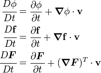
To refresh your memory, recall that the material time derivative is given by
Conservation of mass
For the situation where a body does not gain or lose mass, the balance of mass is written as
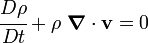
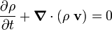
Sometimes, this equation is also written in conservative form as
If the material is incompressible then the density does not change with time and we get

For Lagrangian descriptions we can show that

where  is the initial density.
Conservation of linear momentum
The balance of linear momentum is essentially Newton's second applied to continua. Newton's second law can be written as

where the linear momentum  is given by
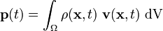
and the total force  is given by
where  is the density,
  is the spatial velocity,
  is
the body force and
is
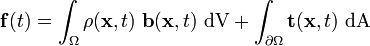
the body force and  is the surface traction. Therefore, the balance
of linear momentum can be written as
is the surface traction. Therefore, the balance
of linear momentum can be written as
![\cfrac{D}{Dt}\left[\int_{\Omega} \rho(\mathbf{x},t)~\mathbf{v}(\mathbf{x},t)~\text{dV}\right] =
\int_{\Omega} \rho(\mathbf{x},t)~\mathbf{b}(\mathbf{x},t)~\text{dV} + \int_{\partial \Omega} \mathbf{t}(\mathbf{x},t)~\text{dA}](../I/m/fa07d2c66b5dddb49f6ffebcb1e49b0e.png)
Now using the transport theorem, we have
![\cfrac{D}{Dt}\left[\int_{\Omega} \rho~\mathbf{v}~\text{dV}\right] =
\int_{\Omega} \left[\rho~\cfrac{D\mathbf{v}}{Dt} +
\left(\cfrac{D\rho}{Dt} + \rho~\boldsymbol{\nabla} \cdot \mathbf{v}\right)\right]~\text{dV}](../I/m/e8b54eaae3dbd3cab1ae8b5bd7cf930f.png)
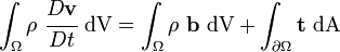
From the conservation of mass, the second term on the right hand side is zero and we are left with
![\cfrac{D}{Dt}\left[\int_{\Omega} \rho(\mathbf{x},t)~\mathbf{v}(\mathbf{x},t)~\text{dV}\right] =
\int_{\Omega} \rho~\cfrac{D\mathbf{v}}{Dt}~\text{dV}](../I/m/cd3bbba33ba0e1a68cfe92e0a1334d4d.png)
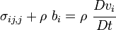
Therefore, the balance of linear momentum can be written as
Using Cauchy's theorem ( ) and the divergence theorem we
can show that the balance of linear momentum can be written as
) and the divergence theorem we
can show that the balance of linear momentum can be written as
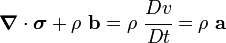
In index notation,
Conservation of angular momentum
We also have to make sure that the moments are balanced. This requirement takes the form of the conservation of angular momentum and can be written as
![\cfrac{D}{Dt}\left[\int_{\Omega} \mathbf{x} \times (\rho~\mathbf{v})~\text{dV}\right] =
\int_{\Omega} \mathbf{x} \times (\rho~\mathbf{b})~\text{dV} + \int_{\partial \Omega} \mathbf{x} \times \mathbf{t}~\text{dA}](../I/m/7b620d41088986a7029fca016d18e0e9.png)
We can show that this equation reduces down to the requirement that the Cauchy stress is symmetric, i.e.,

Conservation of energy
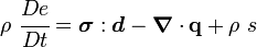
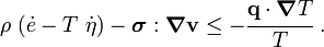
The balance of energy can be expressed as

where  is the internal energy per unit mass,
  is the heat flux vector
and
is the heat flux vector
and  is the heat source per unit volume.
We may also write this equation as
where  , the rate of deformation tensor, is the symmetric part of the
velocity gradient. We can do this because the contraction of the skew
symmetric part of the velocity gradient with the symmetric Cauchy stress gives
us zero.
, the rate of deformation tensor, is the symmetric part of the
velocity gradient. We can do this because the contraction of the skew
symmetric part of the velocity gradient with the symmetric Cauchy stress gives
us zero.
For purely mechanical problems,  and
and  . So we can write
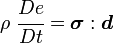
This shows that  and
and  are conjugate in power.
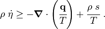
Entropy inequality
The entropy inequality is useful in determining which forms of the constitutive equations are admissible. This inequality is also called the dissipation inequality. In its Clausius-Duhem form, the inequality may written as

where  is the specific entropy (entropy per unit mass) and
  is the
temperature.
is the
temperature.
In differential form the Clausius-Duhem inequality can be written as
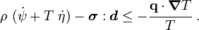
In terms of the specific internal energy, the entropy inequality can be expressed as
If we define the Helmholtz free energy (the energy that is available to do mechanical work) as
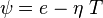
we can also write,
Governing equations in the reference configuration
The Lagrangian form of the governing equations can be obtained using the relations between the various measures in the deformed and reference configurations.
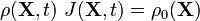
Balance of mass
The Lagrangian form of the balance of mass is
Balance of linear momentum
The Lagrangian form of the balance of linear momentum is
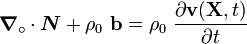
where  is the nominal stress and
  indicates that the
derivatives are with respect to
indicates that the
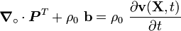
derivatives are with respect to  . In terms of the first Piola-Kirchhoff
stress
. In terms of the first Piola-Kirchhoff
stress  we can write
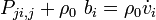
In index notation,
Balance of angular momentum
The balance of angular momentum in Lagrangian form is
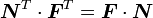
In terms of the first Piola-Kirchhoff stress
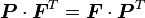
In terms of the second Piola-Kirchhoff stress

Balance of energy
In the material frame, the balance of energy takes the form
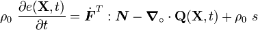
where  is the heat flux per unit reference area.
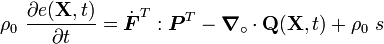
In terms of the first Piola-Kirchhoff stress tensor we have
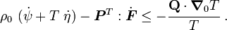
Entropy inequality
The entropy inequality in Lagrangian form is
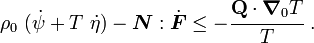
In terms of the first P-K stress we have
Conjugate work measures
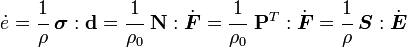
Whatever measures we choose to use to represent stress and strain (or a rate of strain), their product should give us a measure of the work done (or the power spent). This measure should not depend on the chosen measures.
Therefore, the correct combination of stress and strain should be work conjugate or power conjugate. Three commonly used power conjugate stress and rate of strain measures are
- The Cauchy stress () and the rate of deformation ().
- The nominal stress () and the rate of the deformation gradient (
 ).
). - The second P-K stress (
 ) and the rate of the Green strain (
 ).
).
We can show that, in the absence of heat fluxes and sources,
Many more work/power conjugate measures can be found in the literature.