Nonlinear finite elements/Objectivity of constitutive relations
< Nonlinear finite elementsMaterial frame indifference
An important consider in nonlinear finite element analysis is material frame indifference or objectivity of the material response. The idea is that the position of the observer frame should not affect the constitutive relations of a material. You can find more details and a history of the idea in Truesdell and Noll (1992) - sections 17, 18, 19, and 19A. [1]
We have already talked about the objectivity of kinematic quantities and stress rates. Let us now discuss the same ideas with a particular constitutive model in mind.
Hyperelastic materials
A detailed description of thermoelastic materials can be found in Continuum mechanics/Thermoelasticity. In this discussion we will avoid the complications induced by including the temperature.
In the material configuration, a hyperelastic material satisfies two requirements:
- a stored energy function (
 ) exists for the material.
 - the stored energy function depends locally only on the deformation gradient.
Given these requirements, if  is the nominal stress (
 is
the first Piola-Kirchhoff stress tensor), then
is
the first Piola-Kirchhoff stress tensor), then
![\boldsymbol{N}^T(\mathbf{X}, t) = \boldsymbol{P}(\mathbf{X},t) = \rho_0~\frac{\partial W}{\partial \boldsymbol{F}}\left[\mathbf{X}, \boldsymbol{F}(\mathbf{X},t)\right]](../I/m/ea1816657215b85e80ce95cedb6e21af.png)
Objectivity
The stored energy function  is said to be objective or frame indifferent
if
is said to be objective or frame indifferent
if

where  is an orthogonal tensor with
  .
.
This objectivity condition can be achieved only if (in the material configuration)

since  .
.
We can show that
|
Constitutive relations for hyperelastic materials |
Proof:
The stress strain relation for a hyperelastic material is
The chain rule then implies that
for any second order tensor
.
Now, using the product rule of differentiation,
or,
where
is the fourth order identity tensor. Therefore,
Using the identity
we have
Therefore, invoking the arbitrariness of
Since
we have
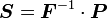
which implies that
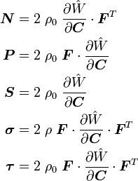
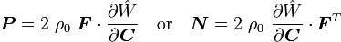
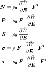
Recall the relations between the 2nd Piola-Kirchhoff stress tensor and the first Piola-Kirchhoff stress tensor (and the nominal stress tensor)
Therefore, we have
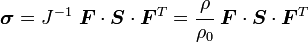
Also from the relation between the Cauchy stress and the 2nd Piola-Kirchhoff stress tensor
we have
![\boldsymbol{P} = \rho_0~\frac{\partial W}{\partial \boldsymbol{F}}\left[\mathbf{X}, \boldsymbol{F}(\mathbf{X},t)\right]](../I/m/3afcfd75f515cef646a2fc78ac72116e.png)


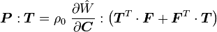

![\frac{\partial \hat{W}}{\partial \boldsymbol{C}}:(\boldsymbol{T}^T\cdot\boldsymbol{F}) =
\left[\boldsymbol{F}\cdot\left(\frac{\partial \hat{W}}{\partial \boldsymbol{C}}\right)^T\right]:\boldsymbol{T}
\quad \text{and} \quad
\frac{\partial \hat{W}}{\partial \boldsymbol{C}}:(\boldsymbol{F}^T\cdot\boldsymbol{T}) =
\left[\boldsymbol{F}\cdot\frac{\partial \hat{W}}{\partial \boldsymbol{C}}\right]:\boldsymbol{T}](../I/m/ecc40df3b144f30c8ff0c3dad2a9ecb1.png)

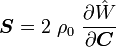
We may also express these relations in terms of the Lagrangian Green strain
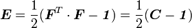
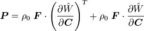
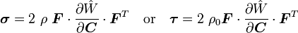
Then we have
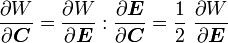
Hence, we can write
|
|
The stored energy function is objective if and only if the Cauchy stress tensor is symmetric, i.e., if the balance of angular momentum holds. Show this.
- ↑ C. Truesdell and W. Noll, 1992, The Nonlinear Field Theories of Mechanics:2nd ed., Springer-Verlag, Berlin