Nonlinear finite elements/Objective stress rates

Objective stress rates

Many constitutive equations are given in rate form as the relation between a stress rate and a strain rate (or the rate of deformation). We would like our constitutive equations to be frame indifferent (objective). If the stress and strain measures are material quantities then objectivity is automatically satisfied. However, if the quantities are spatial, then the objectivity of the stress rate is not guaranteed even if the strain rate is objective.

Under rigid body rotations, the Cauchy stress tensor $\boldsymbol{\sigma}$ transforms as

\boldsymbol{\sigma}_r = \boldsymbol{Q}\cdot\boldsymbol{\sigma}\cdot\boldsymbol{Q}^T ~;~~ \boldsymbol{Q}\cdot\boldsymbol{Q}^T = \boldsymbol{\mathit{1}}

Since $\boldsymbol{\sigma}$ is a spatial quantity and the transformation follows the rules of tensor transformations, $\boldsymbol{\sigma}$ is objective.

However,

\cfrac{d}{dt}(\boldsymbol{\sigma}_r) = \dot{\boldsymbol{\sigma}}_r = \dot{\boldsymbol{Q}}\cdot\boldsymbol{\sigma}\cdot\boldsymbol{Q}^T + \boldsymbol{Q}\cdot\dot{\boldsymbol{\sigma}}\cdot\boldsymbol{Q}^T + \boldsymbol{Q}\cdot\boldsymbol{\sigma}\cdot\dot{\boldsymbol{Q}}^T

or,

\dot{\boldsymbol{\sigma}}_r \ne \boldsymbol{Q}\cdot\dot{\boldsymbol{\sigma}}\cdot\boldsymbol{Q}^T

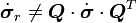
Therefore the stress rate is not objective unless the rate of rotation is zero, i.e. $\boldsymbol{Q}$ is constant.

There are numerous objective stress rates in the literature on continuum mechanics - all of which can be shown to be special forms of Lie derivatives. However, we will focus on three which are widely used.

The Truesdell rate
The Green-Naghdi rate
The Jaumann rate

Truesdell stress rate of the Cauchy stress

The relation between the Cauchy stress and the 2nd P-K stress is called the Piola transformation. Recall that this transformation can be written in terms of the pull-back of $\boldsymbol{\sigma}$ or the push-forward of $\boldsymbol{S}$ as

\boldsymbol{S} = J~\phi^{*}[\boldsymbol{\sigma}] ~;~~ \boldsymbol{\sigma} = J^{-1}~\phi_{*}[\boldsymbol{S}]

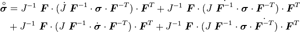
The Truesdell rate of the Cauchy stress is the Piola transformation of the material time derivative of the 2nd P-K stress. We thus define

\overset{\circ}{\boldsymbol{\sigma}} = J^{-1}~\phi_{*}[\dot{\boldsymbol{S}}]

Expanded out, this means that

\overset{\circ}{\boldsymbol{\sigma}} = J^{-1}~\boldsymbol{F}\cdot\dot{\boldsymbol{S}}\cdot\boldsymbol{F}^T = J^{-1}~\boldsymbol{F}\cdot \left[\cfrac{d}{dt}\left(J~\boldsymbol{F}^{-1}\cdot\boldsymbol{\sigma}\cdot\boldsymbol{F}^{-T}\right)\right] \cdot\boldsymbol{F}^T = J^{-1}~\mathcal{L}_\varphi[\boldsymbol{\tau}]

where the Kirchhoff stress $\boldsymbol{\tau} = J~\boldsymbol{\sigma}$ and the Lie derivative of the Kirchhoff stress is

\mathcal{L}_\varphi[\boldsymbol{\tau}] = \boldsymbol{F}\cdot \left[\cfrac{d}{dt}\left(\boldsymbol{F}^{-1}\cdot\boldsymbol{\tau}\cdot\boldsymbol{F}^{-T}\right)\right] \cdot\boldsymbol{F}^T ~.

This expression can be simplified to the well known expression for the Truesdell rate of the Cauchy stress

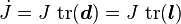
Truesdell rate of the Cauchy stress

\overset{\circ}{\boldsymbol{\sigma}} = \dot{\boldsymbol{\sigma}} - \boldsymbol{l}\cdot\boldsymbol{\sigma} - \boldsymbol{\sigma}\cdot\boldsymbol{l}^T + \text{tr}(\boldsymbol{l})~\boldsymbol{\sigma}

Proof:

We start with

$\overset{\circ}{\boldsymbol{\sigma}} = J^{-1}~\boldsymbol{F}\cdot \left[\cfrac{d}{dt}\left(J~\boldsymbol{F}^{-1}\cdot\boldsymbol{\sigma}\cdot\boldsymbol{F}^{-T}\right)\right] \cdot\boldsymbol{F}^T ~.$

Expanding the derivative inside the square brackets, we get

$\begin{align} \overset{\circ}{\boldsymbol{\sigma}} & = J^{-1}~\boldsymbol{F}\cdot(\dot{J}~\boldsymbol{F}^{-1}\cdot\boldsymbol{\sigma}\cdot\boldsymbol{F}^{-T})\cdot\boldsymbol{F}^T + J^{-1}~\boldsymbol{F}\cdot(J~\dot{\boldsymbol{F}^{-1}}\cdot\boldsymbol{\sigma}\cdot\boldsymbol{F}^{-T})\cdot\boldsymbol{F}^T \\ & + J^{-1}~\boldsymbol{F}\cdot(J~\boldsymbol{F}^{-1}\cdot\dot{\boldsymbol{\sigma}}\cdot\boldsymbol{F}^{-T})\cdot\boldsymbol{F}^T + J^{-1}~\boldsymbol{F}\cdot(J~\boldsymbol{F}^{-1}\cdot\boldsymbol{\sigma}\cdot\dot{\boldsymbol{F}^{-T}})\cdot\boldsymbol{F}^T \end{align}$

or,

$\overset{\circ}{\boldsymbol{\sigma}} = J^{-1}~\dot{J}~\boldsymbol{\sigma} + \boldsymbol{F}\cdot\dot{\boldsymbol{F}^{-1}}\cdot\boldsymbol{\sigma} + \dot{\boldsymbol{\sigma}} + \boldsymbol{\sigma}\cdot\dot{\boldsymbol{F}^{-T}}\cdot\boldsymbol{F}^T$

Now,

$\boldsymbol{F}\cdot\boldsymbol{F}^{-1} = \boldsymbol{\mathit{1}}$

Therefore,

$\cfrac{d}{dt}\left(\boldsymbol{F}\cdot\boldsymbol{F}^{-1}\right) = 0 \quad \implies \quad \dot{\boldsymbol{F}}\cdot\boldsymbol{F}^{-1} + \boldsymbol{F}\cdot\dot{\boldsymbol{F}^{-1}} = 0$

or,

$\dot{\boldsymbol{F}^{-1}} = - \boldsymbol{F}^{-1}\cdot\boldsymbol{l} \quad \implies \quad \dot{\boldsymbol{F}^{-T}} = - \boldsymbol{l}^T\cdot\boldsymbol{F}^{-T}$

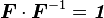
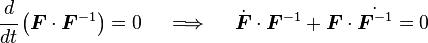
where the velocity gradient $\boldsymbol{l} = \dot{\boldsymbol{F}}\cdot\boldsymbol{F}^{-1}$ .

Also, the rate of change of volume is given by

$\dot{J} = J~\text{tr}(\boldsymbol{d}) = J~\text{tr}(\boldsymbol{l})$

where $\boldsymbol{d}$ is the rate of deformation tensor.

Therefore,

$\overset{\circ}{\boldsymbol{\sigma}} = J^{-1}~J~\text{tr}(\boldsymbol{l})~\boldsymbol{\sigma} - \boldsymbol{F}\cdot\boldsymbol{F}^{-1}\cdot\boldsymbol{l}\cdot\boldsymbol{\sigma} + \dot{\boldsymbol{\sigma}} - \boldsymbol{\sigma}\cdot\boldsymbol{l}^T\cdot\boldsymbol{F}^{-T}\cdot\boldsymbol{F}^T$

or,

$\overset{\circ}{\boldsymbol{\sigma}} = \dot{\boldsymbol{\sigma}} - \boldsymbol{l}\cdot\boldsymbol{\sigma} - \boldsymbol{\sigma}\cdot\boldsymbol{l}^T + \text{tr}(\boldsymbol{l})~\boldsymbol{\sigma}$

You can easily show that the Truesdell rate is objective.

Truesdell rate of the Kirchhoff stress

The Truesdell rate of the Kirchhoff stress can be obtained by noting that

\boldsymbol{S} = \phi^{*}[\boldsymbol{\tau}] ~;~~ \boldsymbol{\tau} = \phi_{*}[\boldsymbol{S}]

and defining

\overset{\circ}{\boldsymbol{\tau}} = \phi_{*}[\dot{\boldsymbol{S}}]

Expanded out, this means that

\overset{\circ}{\boldsymbol{\tau}} = \boldsymbol{F}\cdot\dot{\boldsymbol{S}}\cdot\boldsymbol{F}^T = \boldsymbol{F}\cdot \left[\cfrac{d}{dt}\left(\boldsymbol{F}^{-1}\cdot\boldsymbol{\tau}\cdot\boldsymbol{F}^{-T}\right)\right] \cdot\boldsymbol{F}^T = \mathcal{L}_\varphi[\boldsymbol{\tau}]

Therefore, the Lie derivative of $\boldsymbol{\tau}$ is the same as the Truesdell rate of the Kirchhoff stress.

FFollowing the same process as for the Cauchy stress above, we can show that

Truesdell rate of the Kirchhoff stress

\overset{\circ}{\boldsymbol{\tau}} = \dot{\boldsymbol{\tau}} - \boldsymbol{l}\cdot\boldsymbol{\tau} - \boldsymbol{\tau}\cdot\boldsymbol{l}^T

Green-Naghdi rate of the Cauchy stress

This is a special form of the Lie derivative (or the Truesdell rate of the Cauchy stress). Recall that the Truesdell rate of the Cauchy stress is given by

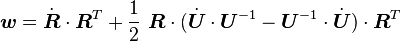
\overset{\circ}{\boldsymbol{\sigma}} = J^{-1}~\boldsymbol{F}\cdot \left[\cfrac{d}{dt}\left(J~\boldsymbol{F}^{-1}\cdot\boldsymbol{\sigma}\cdot\boldsymbol{F}^{-T}\right)\right] \cdot\boldsymbol{F}^T ~.

From the polar decomposition theorem we have

\boldsymbol{F} = \boldsymbol{R}\cdot\boldsymbol{U}

where $\boldsymbol{R}$ is the orthogonal rotation tensor ( $\boldsymbol{R}^{-1} = \boldsymbol{R}^T$ ) and $\boldsymbol{U}$ is the symmetric, positive definite, right stretch.

If we assume that $\boldsymbol{U} = \boldsymbol{\mathit{1}}$ we get $\boldsymbol{F} = \boldsymbol{R}$ . Also since there is no stretch $J = 1$ and we have $\boldsymbol{\tau} = \boldsymbol{\sigma}$ . Note that this doesn't mean that there is not stretch in the actual body - this simplification is just for the purposes of defining an objective stress rate. Therefore

\overset{\circ}{\boldsymbol{\sigma}} = \boldsymbol{R}\cdot \left[\cfrac{d}{dt}\left(\boldsymbol{R}^{-1}\cdot\boldsymbol{\sigma}\cdot\boldsymbol{R}^{-T}\right)\right] \cdot\boldsymbol{R}^T = \boldsymbol{R}\cdot\left[\cfrac{d}{dt}\left(\boldsymbol{R}^T\cdot\boldsymbol{\sigma}\cdot\boldsymbol{R}\right)\right] \cdot\boldsymbol{R}^T

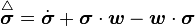
We can show that this expression can be simplified to the commonly used form of the Green-Naghdi rate

Green-Naghdi rate of the Cauchy stress

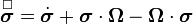
\overset{\square}{\boldsymbol{\sigma}} = \dot{\boldsymbol{\sigma}} + \boldsymbol{\sigma}\cdot\boldsymbol{\Omega} - \boldsymbol{\Omega}\cdot\boldsymbol{\sigma}

where $\boldsymbol{\Omega} = \dot{\boldsymbol{R}}\cdot\boldsymbol{R}^T$ .

The Green-Naghdi rate of the Kirchhoff stress also has the form since the stretch is not taken into consideration, i.e.,

\overset{\square}{\boldsymbol{\tau}} = \dot{\boldsymbol{\tau}} + \boldsymbol{\tau}\cdot\boldsymbol{\Omega} - \boldsymbol{\Omega}\cdot\boldsymbol{\tau}

Proof:

Expanding out the derivative

$\overset{\circ}{\boldsymbol{\sigma}} = \boldsymbol{R}\cdot\dot{\boldsymbol{R}^T}\cdot\boldsymbol{\sigma}\cdot\boldsymbol{R}\cdot\boldsymbol{R}^T + \boldsymbol{R}\cdot\boldsymbol{R}^T\cdot\dot{\boldsymbol{\sigma}}\cdot\boldsymbol{R}\cdot\boldsymbol{R}^T + \boldsymbol{R}\cdot\boldsymbol{R}^T\cdot\boldsymbol{\sigma}\cdot\dot{\boldsymbol{R}}\cdot\boldsymbol{R}^T$

or,

$\overset{\circ}{\boldsymbol{\sigma}} = \boldsymbol{R}\cdot\dot{\boldsymbol{R}^T}\cdot\boldsymbol{\sigma} + \dot{\boldsymbol{\sigma}} + \boldsymbol{\sigma}\cdot\dot{\boldsymbol{R}}\cdot\boldsymbol{R}^T$

Now,

$\boldsymbol{R}\cdot\boldsymbol{R}^T = \boldsymbol{\mathit{1}} \quad \implies \quad \dot{\boldsymbol{R}}\cdot\boldsymbol{R}^T = - \boldsymbol{R}\cdot\dot{\boldsymbol{R}^T}$

Therefore,

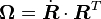
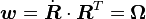
$\overset{\circ}{\boldsymbol{\sigma}} = \dot{\boldsymbol{\sigma}} + \boldsymbol{\sigma}\cdot\dot{\boldsymbol{R}}\cdot\boldsymbol{R}^T - \dot{\boldsymbol{R}}\cdot\boldsymbol{R}^T\cdot\boldsymbol{\sigma}$

If we define the angular velocity as

$\boldsymbol{\Omega} = \dot{\boldsymbol{R}}\cdot\boldsymbol{R}^T$

we get the commonly used form of the Green-Naghdi rate

$\overset{\square}{\boldsymbol{\sigma}} = \dot{\boldsymbol{\sigma}} + \boldsymbol{\sigma}\cdot\boldsymbol{\Omega} - \boldsymbol{\Omega}\cdot\boldsymbol{\sigma}$

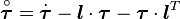
Jaumann rate of the Cauchy stress

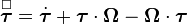
The Jaumann rate of the Cauchy stress is a further specialization of the Lie derivative (Truesdell rate). This rate has the form

Jaumann rate of the Cauchy stress

\overset{\triangle}{\boldsymbol{\sigma}} = \dot{\boldsymbol{\sigma}} + \boldsymbol{\sigma}\cdot\boldsymbol{w} - \boldsymbol{w}\cdot\boldsymbol{\sigma}

where $\boldsymbol{w}$ is the spin tensor.

The Jaumann rate is used widely in computations primarily for two reasons

it is relatively easy to implement.
it leads to symmetric tangent moduli.

Recall that the spin tensor $\boldsymbol{w}$ (the skew part of the velocity gradient) can be expressed as

\boldsymbol{w} = \dot{\boldsymbol{R}}\cdot\boldsymbol{R}^T + \frac{1}{2}~\boldsymbol{R}\cdot(\dot{\boldsymbol{U}}\cdot\boldsymbol{U}^{-1} - \boldsymbol{U}^{-1}\cdot\dot{\boldsymbol{U}})\cdot\boldsymbol{R}^T

Thus for pure rigid body motion

\boldsymbol{w} = \dot{\boldsymbol{R}}\cdot\boldsymbol{R}^T = \boldsymbol{\Omega}

Alternatively, we can consider the case of proportional loading when the principal directions of strain remain constant. An example of this situation is the axial loading of a cylindrical bar. In that situation, since

\boldsymbol{U} = \left[\begin{array}{ccc} \lambda_{X}\\ & \lambda_{Y}\\ & & \lambda_{Z}\end{array}\right]

we have

\dot{\boldsymbol{U}} = \left[\begin{array}{ccc} \dot{\lambda}_{X}\\ & \dot{\lambda}_{Y}\\ & & \dot{\lambda}_{Z}\end{array}\right]

Also,

\boldsymbol{U}^{-1} = \left[\begin{array}{ccc} 1/\lambda_{X}\\ & 1/\lambda_{Y}\\ & & 1/\lambda_{Z}\end{array}\right]

Therefore,

\dot{\boldsymbol{U}}\cdot\boldsymbol{U}^{-1} = \left[\begin{array}{ccc} \dot{\lambda}_{X}/\lambda_{X}\\ & \dot{\lambda}_{Y}/\lambda_{Y}\\ & & \dot{\lambda}_{Z}/\lambda_{Z}\end{array}\right]=U^{-1}\dot{U}

This once again gives

\boldsymbol{w} = \dot{\boldsymbol{R}}\cdot\boldsymbol{R}^T = \boldsymbol{\Omega}

In general, if we approximate

\boldsymbol{w} \approx \dot{\boldsymbol{R}}\cdot\boldsymbol{R}^T

the Green-Naghdi rate becomes the Jaumann rate of the Cauchy stress

\overset{\triangle}{\boldsymbol{\sigma}} = \dot{\boldsymbol{\sigma}} + \boldsymbol{\sigma}\cdot\boldsymbol{w} - \boldsymbol{w}\cdot\boldsymbol{\sigma}

Other objective stress rates

There can be an infinite variety of objective stress rates. One of these is the Oldroyd stress rate

\overset{\triangledown}{\boldsymbol{\sigma}} = \mathcal{L}_\varphi[\boldsymbol{\sigma}] = \boldsymbol{F}\cdot\left[\cfrac{d}{dt}\left(\boldsymbol{F}^{-1}\cdot\boldsymbol{\sigma}\cdot\boldsymbol{F}^{-T}\right) \right]\cdot\boldsymbol{F}^T

In simpler form, the Oldroyd rate is given by

\overset{\triangledown}{\boldsymbol{\sigma}} = \dot{\boldsymbol{\sigma}} - \boldsymbol{l}\cdot\boldsymbol{\sigma} - \boldsymbol{\sigma}\cdot\boldsymbol{l}^T

If the current configuration is assumed to be the reference configuration then the pull back and push forward operations can be conducted using $\boldsymbol{F}^T$ and $\boldsymbol{F}^{-T}$ respectively. The Lie derivative of the Cauchy stress is then called the convective stress rate

\overset{\diamond}{\boldsymbol{\sigma}} = \boldsymbol{F}^{-T}\cdot\left[\cfrac{d}{dt}\left(\boldsymbol{F}^T\cdot\boldsymbol{\sigma}\cdot\boldsymbol{F}\right) \right]\cdot\boldsymbol{F}^{-1}

In simpler form, the convective rate is given by

\overset{\diamond}{\boldsymbol{\sigma}} = \dot{\boldsymbol{\sigma}} + \boldsymbol{l}\cdot\boldsymbol{\sigma} + \boldsymbol{\sigma}\cdot\boldsymbol{l}^T

Caveat on objective stress rates

The following figure shows the performance of various objective rates in a pure shear test where the material model is a hypoelastic one with constant elastic moduli. The ratio of the shear stress to the displacement is plotted as a function of time. The same moduli are used with the three objective stress rates.

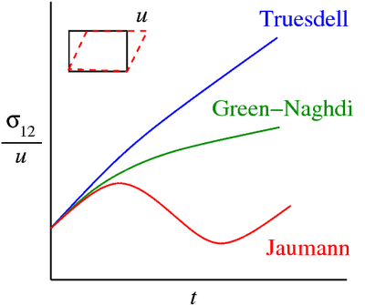Predictions from three objective stress rates under shear

Clearly there are spurious oscillations observed for the Jaumann stress rate. This is not because one rate is better than another but because its is a misuse of material models to use the same constants with different objective rates.

For this reason, a recent trend has been to avoid objective stress rates altogether where possible.

This article is issued from Wikiversity - version of the Monday, June 10, 2013. The text is available under the Creative Commons Attribution/Share Alike but additional terms may apply for the media files.