Nonlinear finite elements/Nonlinear axially loaded bar
< Nonlinear finite elementsAn Example: Axial Bar with Distributed Load
Recall the bar with a distributed axial body load from Handout 8 (see Figure 1).
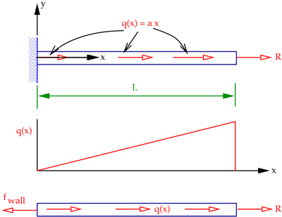 Figure 1. Distributed axial loading of a bar. |
In our previous discussion we had assumed that the bar had a constant Young's modulus of  , that is, the constitutive model of the bar was linear elastic.
Let us now assume that the stress-strain relationship is nonlinear, and of the form
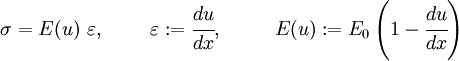
where  is a material constant which can be interpreted as the initial Young's modulus. Figure 2 shows
how the stress-strain relationship for this material looks.
is a material constant which can be interpreted as the initial Young's modulus. Figure 2 shows
how the stress-strain relationship for this material looks.
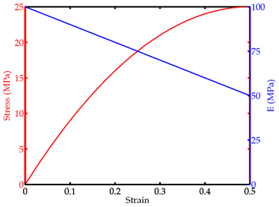 Figure 2. Stress-strain relationship for the nonlinear bar. |
The governing differential equation for the bar is
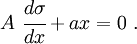
If we plug in the stress-strain relation into the governing equation, we get
![{
A~\cfrac{d}{dx}\left[E(u)\cfrac{du}{dx}\right] + ax = 0 ~.
}](../I/m/dbb1480fc327297e9111f9eb984f2aad.png)
Notice that we have not included the expression for  in the above equation. The reason is that we want to maintain the symmetry of the stiffness matrix.
Effect of including expression for
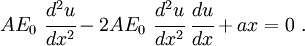
You can see what happens when we include the expression for in the steps below. We get,
![A~\cfrac{d}{dx}\left[E_0\left(1-\cfrac{du}{dx}\right)
\cfrac{du}{dx}\right] + ax = 0 ~.](../I/m/740ad3130377079ced1ef86a115a8aa3.png)
or,
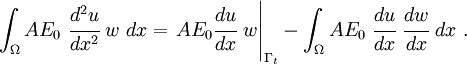
Now, when we try to derive the weak form, we get

The first integral is the same as before, and we get
The third integral remains the same. However, the second integral becomes
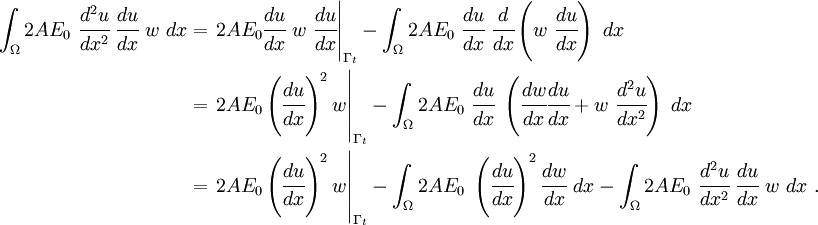
Rearranging, we get
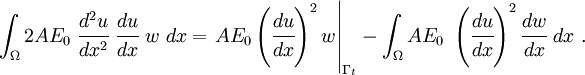
After collecting all the terms, the weak form becomes

Separating the terms corresponding to the internal and external forces, we get
![\int_{\Omega} AE_0~\cfrac{du}{dx}~\cfrac{dw}{dx}~dx -
\int_{\Omega} AE_0~\left(\cfrac{du}{dx}\right)^2\cfrac{dw}{dx}~dx
= \int_{\Omega} ax~w~dx +
\left. AE_0\left[\cfrac{du}{dx} -
\left(\cfrac{du}{dx}\right)^2\right]w\right|_{\Gamma_t}~.](../I/m/8838491afa25c468ac61b76c2828fc66.png)
If we choose trial and weighting functions
and plug them into the weak form, we get
![\int_{\Omega}
AE_0\left(\sum_j u_j\cfrac{dN_j}{dx}\right)\cfrac{dN_i}{dx}~dx -
\int_{\Omega} AE_0~\left(\sum_j u_j\cfrac{dN_j}{dx}\right)^2
\cfrac{dN_i}{dx}~dx
= \int_{\Omega} ax~N_i~dx +
\left. AE_0\left[\cfrac{du}{dx} -
\left(\cfrac{du}{dx}\right)^2\right]w\right|_{\Gamma_t}~.](../I/m/e2a885511256d5ee242af2d94807ccd9.png)
Taking the constants out of the integrals, we get (regarding this step, read the Discuss page of this article)
![AE_0 \sum_j \left[\int_{\Omega}
\left(\cfrac{dN_j}{dx}\cfrac{dN_i}{dx} -
\left(\cfrac{dN_j}{dx}\right)^2\cfrac{dN_i}{dx}\right)~dx \right]u_j
= \int_{\Omega} ax~N_i~dx +
\left. AE_0\left[\cfrac{du}{dx} -
\left(\cfrac{du}{dx}\right)^2\right]w\right|_{\Gamma_t}~.](../I/m/dd5dac62c80edea1c928f7a8db4f3c87.png)
Therefore, the coefficients of the stiffness matrix are given by
![K_{ij} = AE_0 \int_{\Omega}
\left[\cfrac{dN_i}{dx}\cfrac{dN_j}{dx} -
\cfrac{dN_i}{dx}\left(\cfrac{dN_j}{dx}\right)^2\right]~dx ~.](../I/m/7d2cb5b55b2bb0ad818718faf2a02be3.png)
This stiffness matrix is not symmetric because of the second term inside the integral. That is,  .
.
We would like to work with a symmetric stiffness matrix for computational reasons, i.e., the amount of storage needed is smaller and there are a number of very fast solvers for symmetric matrices.