Nonlinear finite elements/Nonlinear axial bar weak form
< Nonlinear finite elementsSymmetric weak form for the axially loaded bar
Let us start with the weak form and derive a symmetric stiffness matrix. We have,
![{
A~\cfrac{d}{dx}\left[E(u)\cfrac{du}{dx}\right] + ax = 0 ~.
}](../I/m/dbb1480fc327297e9111f9eb984f2aad.png)
Once again, we multiply with a weighting function and integrate over an element to get
![\int_{\Omega} A~\cfrac{d}{dx}\left[E(u)\cfrac{du}{dx}\right]w~dx +
\int_{\Omega} axw = 0 ~.](../I/m/43ae9333d91dc6b4dbf1ad44ad57540a.png)
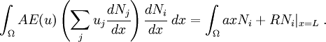
Integrating the first term by parts, we get
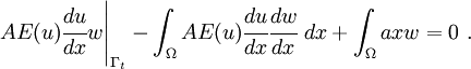
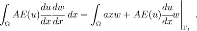
Taking the internal force terms to the left and the external force terms to the right, we get
Note that, at  ,
,
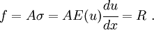
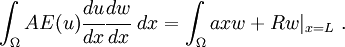
Also, at  , we have
  . The external surface force is zero at all other points. Therefore,
The finite element approximation
Let, the trial and weighting functions be
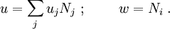
Then, we get
Take the constants outside the integral sign as usual, and we can write
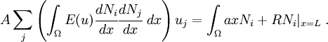
The above can be written in the usual form as

where
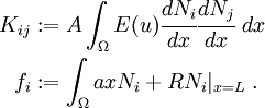
This stiffness matrix is symmetric. However, we are still left with the problem of dealing with the  part.
part.
Dealing with
The expression of is
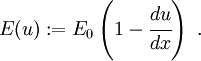
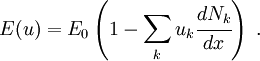
In terms of the trial function, we have
I have chosen to call the index  in order to distinguish it from the index names that we have already used, that is
  and
and  .
.
Plugging the expansion for into the expression for  we get
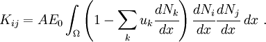
Notice that the stiffness matrix continues to remain symmetric when we do this because the sum over includes all the relevant nodes.
The stiffness matrix is now a function of the unknown displacements  and the system of equations can be written as
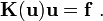
This is a nonlinear system of equations and cannot be solved directly (as was done for linear systems).
Making things a bit more concrete
Let us get a bit more explicit about what all that leads to.
Assume that the bar is divided into two linear elements. Therefore, there are three global nodes:  ,
,  , and
, and  . Each element has two nodes which have local numbers and .
The shape functions within each element are
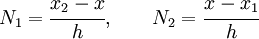
where  is the coordinate of node of the element, and
  is the coordinate of node of the element. The length of the element is
  .
.
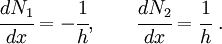
The derivatives of the shape functions are
The element stiffness matrix terms can be written as
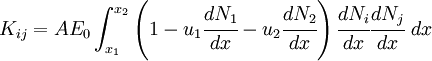
where  is the displacement of local node , and
  is the displacement of local node .
Plugging in the values of the derivatives of the shape functions, we get
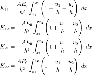
The terms inside the integrals are the same for all the coefficients of the stiffness matrix (this is not true in general), and we have
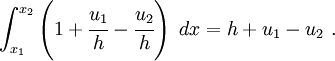
Therefore,
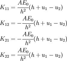
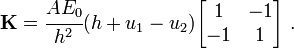
In matrix form, the element stiffness matrix is
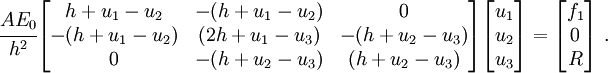
For simplicity, let us set the body force term  to zero. Let us also assume that both elements have equal lengths. Then the assembled global system of equations (for the two element mesh) is
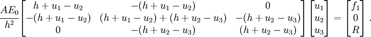
After simplification, we have
The stiffness matrix is a function of , , and  .
.
The boundary condition at is  . Therefore, the reduced system of equations can be written as
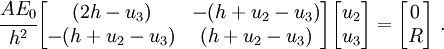
The reduced stiffness matrix is a function of and .
How can we find and under these circumstances? We will use the Newton-Raphson numerical technique.