Nonlinear finite elements/Newton method for finite elements
< Nonlinear finite elementsNewton's method for nonlinear finite elements
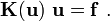
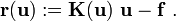
The finite element system of equations is of the form
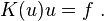
In order to write it in the form  , we define the residual

Then, the Newton iteration formula becomes
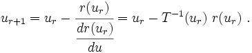
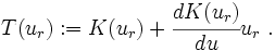
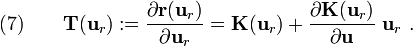
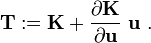
The slope of the tangent (the tangent stiffness) is
![\begin{align}
T(u_r) := \cfrac{dr(u_r)}{du}
& = \cfrac{d}{du}[K(u) u - f]\ \\
& = K(u) + \cfrac{dK(u)}{du}u\ \\
& = K(u_r) + \cfrac{dK(u_r)}{du}u_r
\end{align}](../I/m/9b0271c484706ddef1492d5b33b01907.png)
Therefore the tangent stiffness is
So far we have considered Newton's method only for single equations. What changes have to be made for a system of equations such as the ones encountered in FEM?
Newton's method for a system of equations
For a system of equations, all we have to do is a straightforward extension of the method as it applies to one dimension. In this case, it's easier to think in terms of matrices instead of individual coefficients of the matrices. Thus, we have
The residual is defined as
Then, the Newton iteration formula is
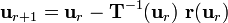
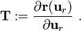
where the tangent stiffness matrix is given by
The iterative procedure is terminated when either the residual is very small or the difference between successive solutions is less than a specified tolerance.
However, both the residual  and the solution
  are vectors. We usually compare the
  (Euclidean) norm of the vectors with a tolerance
  . In symbolic form, we check the norm of the residual using
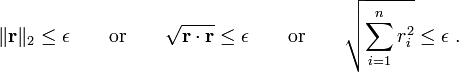
For the difference between successive solutions we check

How do we calculate the derivative of  with respect to ?
In equation (7) we have a terms that involves a partial derivative of matrix with respect to the vector . To see what that means, let us look at the component form of the tangent stiffness matrix.
The tangent stiffness matrix is defined as
Let us consider a  stiffness matrix and see what the above equation means. The residual is
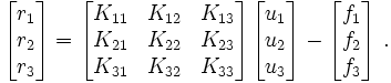
Expanding the above matrix equation out we get
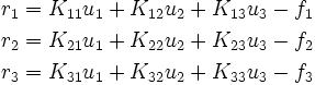
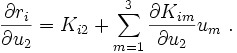
Taking derivatives with respect to  , we get

In shorter form, we can write

Similarly, taking derivatives with respect to  , we get
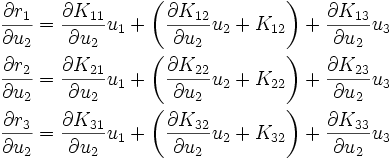
The short form of the above is
Finally, taking derivatives with respect to  gives us
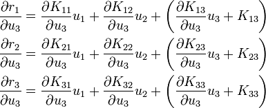
The short form is

Combining the three short forms of the 9 equations, we get
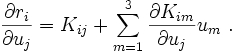
Each of these terms represents one component  of the matrix
  ,
and for a
,
and for a  stiffness matrix we get
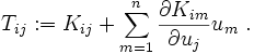
In matrix notation, the above equation is written as
This shows us how to compute the derivative of with respect to and hence .
Note that we can form the tangent stiffness matrix over an element and assemble the contributions from each element to get the global tangent stiffness matrix. The reasons are the same as those for the standard global stiffness matrix.