Nonlinear finite elements/Matrices
< Nonlinear finite elementsMuch of finite elements revolves around forming matrices and solving systems of linear equations using matrices. This learning resource gives you a brief review of matrices.
Matrices
Suppose that you have a linear system of equations
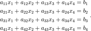
Matrices provide a simple way of expressing these equations. Thus, we can instead write
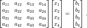
An even more compact notation is
![\left[\mathsf{A}\right] \left[\mathsf{x}\right] = \left[\mathsf{b}\right] ~~~~\text{or}~~~~ \mathbf{A} \mathbf{x} = \mathbf{b} ~.](../I/m/9ab65143e05a0e68423b953fbc300fc3.png)
Here  is a
is a  matrix while
  and
and  are
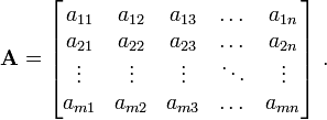
are  matrices. In general, an
  matrix is a set of numbers
arranged in
matrix is a set of numbers
arranged in  rows and
  columns.
Practice Exercises
Practice: Expressing Linear Equations As Matrices
Types of Matrices
Common types of matrices that we encounter in finite elements are:
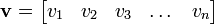
- a row vector that has one row and columns.
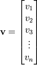
- a column vector that has rows and one column.
- a square matrix that has an equal number of rows and columns.
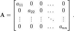
- a diagonal matrix which is a square matrix with only the
diagonal elements ( ) nonzero.
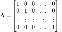
- the identity matrix (
 ) which is a diagonal matrix and
with each of its nonzero elements () equal to 1.
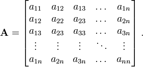
- a symmetric matrix which is a square matrix with elements
such that  .
.
- a skew-symmetric matrix which is a square matrix with elements
such that  .
.
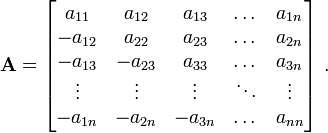
Note that the diagonal elements of a skew-symmetric matrix have to be zero:  .
.
Matrix addition
Let and  be two matrices with components
  and
and  , respectively. Then

Multiplication by a scalar
Let be a matrix with components and let
 be a scalar quantity. Then,

Multiplication of matrices
Let be a matrix with components . Let be a  matrix with components .
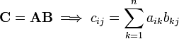
The product  is defined only if
  . The matrix
  is a
is a  matrix with components
  . Thus,
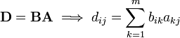
Similarly, the product  is defined only if
  . The matrix
  is a
is a  matrix with components
  . We have
Clearly,  in general, i.e., the matrix product is not
commutative.
in general, i.e., the matrix product is not
commutative.
However, matrix multiplication is distributive. That means

The product is also associative. That means

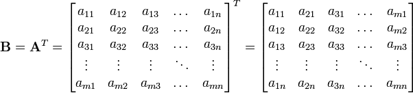
Transpose of a matrix
Let be a matrix with components . Then the transpose of the matrix is defined as the  matrix
  with components
  . That is,
An important identity involving the transpose of matrices is

Determinant of a matrix
The determinant of a matrix is defined only for square matrices.
For a  matrix , we have

For a  matrix, the determinant is calculated by expanding into
minors as
matrix, the determinant is calculated by expanding into
minors as
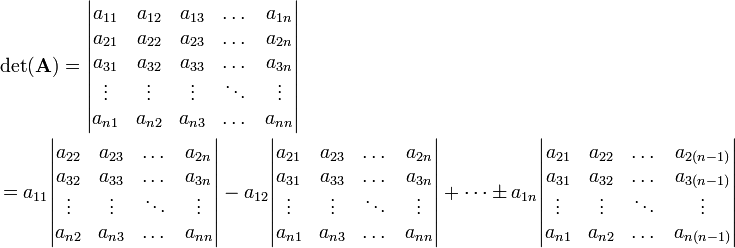
In short, the determinant of a matrix has the value
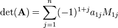
where  is the determinant of the submatrix of formed
by eliminating row
is the determinant of the submatrix of formed
by eliminating row  and column
  from .
Some useful identities involving the determinant are given below.
- If is a matrix, then

- If is a constant and is a matrix, then

- If and are two matrices, then

If you think you understand determinants, take the quiz.
Inverse of a matrix
Let be a matrix. The inverse of is denoted by  and is defined such that

where is the identity matrix.
The inverse exists only if  . A singular matrix
does not have an inverse.
. A singular matrix
does not have an inverse.
An important identity involving the inverse is

since this leads to:

Some other identities involving the inverse of a matrix are given below.
- The determinant of a matrix is equal to the multiplicative inverse of the
determinant of its inverse.

- The determinant of a similarity transformation of a matrix
is equal to the original matrix.

We usually use numerical methods such as Gaussian elimination to compute the inverse of a matrix.
Eigenvalues and eigenvectors
A thorough explanation of this material can be found at Eigenvalue, eigenvector and eigenspace. However, for further study, let us consider the following examples:
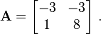
- Let :
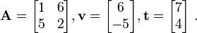
Which vector is an eigenvector for ?
We have
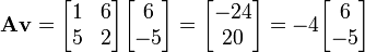 , and
, and 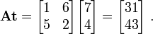
Thus,  is an eigenvector.
- Is
 an eigenvector for
  ?
?
We have that since 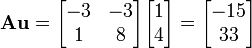 , is not an eigenvector for