Nonlinear finite elements/Kinematics - time derivatives and rates
< Nonlinear finite elementsTime derivatives and rate quantities
Material time derivatives
Material time derivatives are needed for many updated Lagrangian formulations of finite element analysis.
Recall that the motion can be expressed as

If we keep  fixed, then the velocity is given by
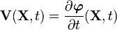
This is the material time derivative expressed in terms of .
The spatial version of the velocity is
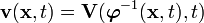
We will use the symbol  for velocity from now on by slightly abusing the
notation.
for velocity from now on by slightly abusing the
notation.
We usually think of quantities such as velocity and acceleration as spatial
quantities which are functions of  (rather than material quantities which
are functions of ).
(rather than material quantities which
are functions of ).
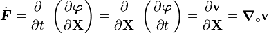
Given the spatial velocity  , if we want to find the acceleration
we will have to consider the fact that
, if we want to find the acceleration
we will have to consider the fact that  , i.e., the
position also changes with time. We do this by using the chain rule. Thus
, i.e., the
position also changes with time. We do this by using the chain rule. Thus

Such a derivative is called the material time derivative expressed
in terms of . The second term in the expression is called the
convective derivative..
Velocity gradient
Let the velocity be expressed in spatial form, i.e., .
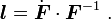
The spatial velocity gradient tensor is given by
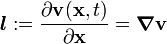
The velocity gradient  is a second order tensor which can expressed as
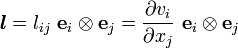
The velocity gradient is a measure the relative velocity of two points in the current configuration.
Time derivative of the deformation gradient
Recall that the deformation gradient is given by

The time derivative of  (keeping fixed) is
Using the chain rule
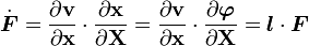
Form this we get the important relation
Time derivative of strain
Let  and
and  be two infinitesimal material line segments in a
body. Then
be two infinitesimal material line segments in a
body. Then

Hence,

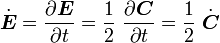
Taking the derivative with respect to  gives us

The material strain rate tensor is defined as
Clearly,
Also,

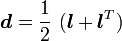
The spatial rate of deformation tensor or stretching tensor is defined as
In fact, we can show that  is the symmetric part of the velocity
gradient, i.e.,
is the symmetric part of the velocity
gradient, i.e.,
For rigid body motions we get  .
.
Lie derivatives
Most of the operations above can be interpreted as push-forward and pull-back operations. Also, time derivatives of these tensors can be interpreted as Lie derivatives.
Recall that the push-forward of the strain tensor from the material configuration to the spatial configuration is given by
![\boldsymbol{e} = \phi_{*} [\boldsymbol{E}] = \boldsymbol{F}^{-T}\cdot\boldsymbol{E}\cdot\boldsymbol{F}^{-1}](../I/m/0ca7cee115e1f24752733434066a1b67.png)
The pull-back of the spatial strain tensor to the material configuration is given by
![\boldsymbol{E} = \phi^{*} [\boldsymbol{e}] = \boldsymbol{F}^T \cdot \boldsymbol{e} \cdot \boldsymbol{F}](../I/m/eaf58e125bce7318d5f29545cc3a6f04.png)
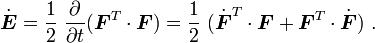
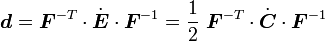
Therefore, the rate of deformation tensor is a push-forward of the material strain rate tensor, i.e.,
![\boldsymbol{d} = \boldsymbol{F}^{-T}\cdot\dot{\boldsymbol{E}}\cdot\boldsymbol{F}^{-1} = \phi_{*}[\dot{\boldsymbol{E}}]](../I/m/8adeb76bc5d7c0726e49a75c6c4b9705.png)
Similarly, the material strain rate tensor is a pull-back of the rate of deformation tensor to the material configuration, i.e.,
![\dot{\boldsymbol{E}} = \boldsymbol{F}^T \cdot \boldsymbol{d} \cdot \boldsymbol{F} = \phi^{*} [\boldsymbol{d}]](../I/m/a2eacc5d546411dd40230f94cbbfe99a.png)
Now,
![\boldsymbol{E} = \phi^{*}[\boldsymbol{e}] \quad \implies \quad
\dot{\boldsymbol{E}} = \frac{\partial }{\partial t} \left(\phi^{*}[\boldsymbol{e}]\right)](../I/m/5df6bcf97762869a75c42799dcbac1fa.png)
Also,
![\boldsymbol{d} = \phi_{*}[\dot{\boldsymbol{E}}] = \phi_{*}
\left[\frac{\partial }{\partial t} \left(\phi^{*}[\boldsymbol{e}]\right)\right]](../I/m/f6a2e89f49f74dae8a5bfcfc49bfc925.png)
Therefore the rate of deformation tensor can be obtained by first pulling
back  to the reference configuration, taking a material time
derivative in that configuration, and then pushing forward the result to
the current configuration.
to the reference configuration, taking a material time
derivative in that configuration, and then pushing forward the result to
the current configuration.
Such an operation is called a Lie derivative. In general, the Lie
derivative of a spatial tensor  is defined as
![\mathcal{L}_{\phi}[\boldsymbol{g}] := \phi_{*}
\left[\frac{\partial }{\partial t} \left(\phi^{*}[\boldsymbol{g}]\right)\right] ~.](../I/m/339fddb1bce0f4ee9c2d2fc27f579cc2.png)
Spin tensor
The velocity gradient tensor can be additively decomposed into a symmetric part and a skew part:
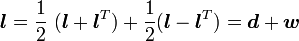
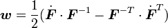
We have seen that is the rate of deformation tensor. The quantity
 is called the spin tensor.
Note that is symmetric while is skew symmetric, i.e.,
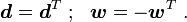
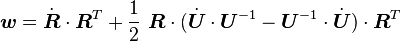
So see why is called a "spin", recall that

Therefore,
Also,

Therefore,

and

So we have

Now

Therefore
The second term above is invariant for rigid body motions and zero for an
uniaxial stretch. Hence, we are left with just a rotation term. This is
why the quantity is called a spin.
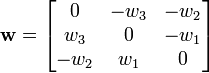
The spin tensor is a skew-symmetric tensor and has an associated axial vector
 (also called the angular velocity vector) whose components are
given by
(also called the angular velocity vector) whose components are
given by

where
The spin tensor and its associated axial vector appear in a number of modern numerical algorithms.
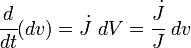
Rate of change of volume
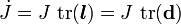
Recall that

Therefore, taking the material time derivative of  (keeping fixed),
we have
(keeping fixed),
we have
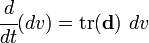
At this stage we invoke the following result from tensor calculus:
If
is an invertible tensor which depends on
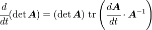
In the case where 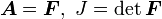 we have
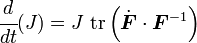
or,
Therefore,
Alternatively, we can also write
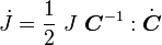
These relations are of immense use in numerical algorithms - particularly
those which involved incompressible behavior, i.e., when  .
.