Nonlinear finite elements/Kinematics - polar decomposition
< Nonlinear finite elementsPolar decomposition
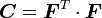
The w:Polar decomposition theorem states that any second order tensor whose determinant is positive can be decomposed uniquely into a symmetric part and an orthogonal part.
In continuum mechanics, the deformation gradient  is such a tensor
because
is such a tensor
because  . Therefore we can write

where  is an orthogonal tensor (
 ) and
) and  are symmetric tensors (
 and
and  ) called the
right stretch tensor and the left stretch tensor, respectively.
This decomposition is called the polar decomposition of .
) called the
right stretch tensor and the left stretch tensor, respectively.
This decomposition is called the polar decomposition of .
Recall that the right Cauchy-Green deformation tensor is defined as
Clearly this is a symmetric tensor. From the polar decomposition of
we have

If you know  then you can calculate
  and hence using
 .
.
How do you find the square root of a tensor?
If you want to find given you will need to take the square root of . How does one do that?
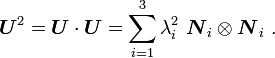
We use what is called the spectral decomposition or eigenprojection of . The spectral decomposition involves expressing in terms of its eigenvalues and eigenvectors. The tensor product of the eigenvectors acts as a basis while the eigenvalues give the magnitude of the projection.
Thus,
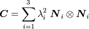
where  are the principal values (eigenvalues) of and
  are the principal directions (eigenvectors) of .
Therefore,
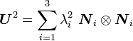
Since the basis does not change, we then have
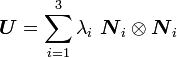
Therefore the  can be interpreted as principal stretches and
the vectors are the directions of the principal stretches.
can be interpreted as principal stretches and
the vectors are the directions of the principal stretches.
Exercise:
If
show that
Example of polar decomposition
Let us assume that the motion is given by
![\begin{align}
x_1 &= \cfrac{1}{4} \left[4~X_1 + (9 - 3~X_1 - 5~X_2 - X_1~X_2)~t\right] \\
x_2 &= X_2 + (4 + 2~X_1)~t
\end{align}](../I/m/a8500c1db5164baa385635977fb116a2.png)
The adjacent figure shows how a unit square subjected to this motion evolves over time.
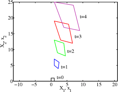 An example of a motion. |
Deformation gradient
The deformation gradient is given by
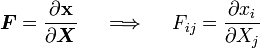
Therefore
![\begin{align}
F_{11} &= \frac{\partial x_1}{\partial X_1} = \cfrac{1}{4}\left[4 + (- 3 - X_2)~t\right] \\
F_{12} &= \frac{\partial x_1}{\partial X_2} = \cfrac{1}{4}\left[(- 5 - X_1)~t\right] \\
F_{21} &= \frac{\partial x_2}{\partial X_1} = 2~t \\
F_{22} &= \frac{\partial x_2}{\partial X_2} = 1
\end{align}](../I/m/c39a96d1d5a09b49f15e3058348641e0.png)
At  at the position
  we have
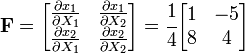
You can calculate the deformation gradient at other points in a similar manner.
Right Cauchy-Green deformation tensor
We have
Therefore,
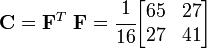
To compute we have to find the eigenvalues and eigenvectors of .
The eigenvalue problem is

where

To find the eigenvalues we solve the characteristic equation
Plugging in the numbers, we get
or
This equation has two solutions
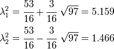
Taking the square roots we get the values of the principal stretches

To compute the eigenvectors we plug into the eigenvalues into the eigenvalue problem to get
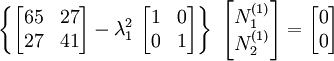
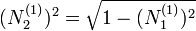
Because this system of equations is not linearly independent, we need another equation to solve this system of equations for  and
and  .
This problem is eliminated by using the following equation (which implies that
.
This problem is eliminated by using the following equation (which implies that  is a unit vector)
Solving, we get
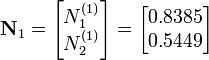
We can do the same thing for the other eigenvector  to get
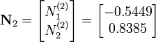
Therefore,

and

Therefore,

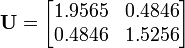
We usually don't see any problem to calculate at this point and go straight to the right stretch tensor.
Right stretch
The right stretch tensor is given by

or
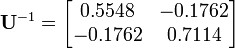
We can invert this matrix to get
Rotation
We can now find the rotation matrix by using th relation
In matrix form,

You can check whether this matrix is orthogonal by seeing whether
 .
.
You thus get the polar decomposition of . In an actual calculation you have to be careful about floating point errors. Otherwise you might not get a matrix that is orthogonal.