Nonlinear finite elements/Homework 11

Problem 1: Small Strain Elastic-Plastic Behavior

For small strains, the strain tensor is given by

\boldsymbol{\varepsilon} = \frac{1}{2}\left[\boldsymbol{\nabla} \mathbf{u} + (\boldsymbol{\nabla} \mathbf{u})^T\right] \qquad\text{or}\qquad \varepsilon_{ij} = \frac{1}{2}(u_{i,j} + u_{j,i}) ~.

In classical (small strain) rate-independent plasticity we start off with an additive decomposition of the strain tensor

\boldsymbol{\varepsilon} = \boldsymbol{\varepsilon}^e + \boldsymbol{\varepsilon}^p \qquad\text{or}\qquad \varepsilon_{ij} = \varepsilon_{ij}^e + \varepsilon_{ij}^p ~.

Assuming linear elasticity, we have the following elastic stress-strain law

\boldsymbol{\sigma} = \boldsymbol{\mathsf{C}} : \boldsymbol{\varepsilon}^e \qquad\text{or}\qquad \sigma_{ij} = C_{ijkl}\varepsilon_{kl}^e ~.

Let us assume that the $J_2$ theory applies during plastic deformation of the material. Hence, the material obeys an associated flow rule

\text{(1)} \qquad \dot{\boldsymbol{\varepsilon}}^p = \dot{\gamma}\frac{\partial f(\boldsymbol{\sigma},\alpha,T)}{\partial \boldsymbol{\sigma}}

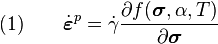
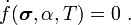
where $\dot{\gamma}$ is the plastic flow rate, $f$ is the yield function, $T$ is the temperature, and $\alpha$ is an internal variable.

Answer the following questions. Show your derivations in a clear and step-by-step manner.

Part 1

Let $\alpha$ be the equivalent plastic strain, defined as

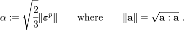
\alpha := \sqrt{\cfrac{2}{3}} \lVert\boldsymbol{\varepsilon}^p\rVert \qquad \text{where} \qquad \lVert\mathbf{a}\rVert = \sqrt{\mathbf{a}:\mathbf{a}} ~.

Express the time derivative of $\alpha$ in terms of $\dot{\gamma}$ and $\partial f/\partial \boldsymbol{\sigma}$ . This is the evolution law for $\alpha$ .

Part 2

For an adiabatic process, the rate of change of temperature can be written as

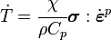
\dot{T} = \cfrac{\chi}{\rho C_p} \boldsymbol{\sigma}:\dot{\boldsymbol{\varepsilon}}^p

where $\chi$ is the Taylor-Quinney coefficient, $\rho$ is the density, and $C_p$ is the specific heat. Express $\dot{T}$ in terms of $\dot{\gamma}$ and $\partial f/\partial \boldsymbol{\sigma}$ . This is the evolution law for $T$ .

Part 3

Write down the rate form of the elastic stress-strain law. Assume that deformations are small so that objectivity of the rates is not a concern.

Part 4

The consistency condition during plastic flow requires that

\dot{f}(\boldsymbol{\sigma}, \alpha, T) = 0 ~.

Write down an expression for the time derivative of $f(\boldsymbol{\sigma},\alpha,T)$ using the chain rule.

Part 5

Use the consistency condition and the expressions you have derived in the previous parts to derive an expression for $\dot{\gamma}$ in terms of $\partial f/\partial\boldsymbol{\sigma}$ , $\partial f/\partial\alpha$ , $\partial f/\partial T$ , $\boldsymbol{\mathsf{C}}$ , and $\dot{\boldsymbol{\varepsilon}}$ .

Part 6

The continuum elastic-plastic tangent modulus is defined by the following relation

\dot{\boldsymbol{\sigma}} = \boldsymbol{\mathsf{C}}^{\text{ep}}:\dot{\boldsymbol{\varepsilon}} ~.

Derive an expression for the elastic plastic tangent modulus using the results you have derived in the previous parts.

Part 7

The $J_2$ theory of plasticity also states that the material satisfies the von Mises yield condition

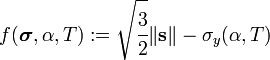
f(\boldsymbol{\sigma},\alpha,T) := \sqrt{\cfrac{3}{2}}\lVert\mathbf{s}\rVert_{} - \sigma_y(\alpha,T)

where $\mathbf{s}$ is the deviatoric part of the stress $\boldsymbol{\sigma}$ . Derive an expression for $\partial f/\partial\boldsymbol{\sigma}$ in terms of the normal to the yield surface

\mathbf{n} = \cfrac{\mathbf{s}}{\lVert\mathbf{s}\rVert_{}} ~.

Part 8

The yield stress $\sigma_y$ is given by the Johnson-Cook model

\sigma_y(\alpha,T) = \left[\sigma_0 + B \alpha^n\right] \left[1 - \left(\cfrac{T - T_0}{T_m -T_0}\right)\right]

where $\sigma_0$ is the initial yield stress, $B, n$ are constants, $T_0$ is a reference temperature, and $T_m$ is the melt temperature. Derive expressions for $\partial f/\partial \alpha$ , and $\partial f/\partial T$ for the von Mises yield condition with the Johnson-Cook flow stress model.

Part 9

Assume that the elastic response of the material is linear, i.e.,

\boldsymbol{\mathsf{C}} = \lambda\boldsymbol{\mathit{1}}\otimes\boldsymbol{\mathit{1}} + 2\mu\boldsymbol{I} ~.

Derive the expression for the elastic-plastic tangent modulus for a von Mises yield condition with Johnson-Cook flow stress for a linear elastic material using the expressions that you have derived in the previous parts.

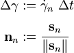
Part 10

Discretize the equations for $\dot{\mathbf{e}}^p$ (equation 1), $\dot{\alpha}$ (from part 1), and $\dot{T}$ (from part 2) using Forward Euler. Use the following notation in your discretized equations:

\begin{align} \Delta\gamma & := \dot{\gamma}_n~\Delta t \\ \mathbf{n}_{n} & := \cfrac{\mathbf{s}_n}{\lVert\mathbf{s}_n\rVert_{}} \end{align}

where $\Delta t$ is the time step, $\dot{\gamma}_n$ is the value of $\dot{\gamma}$ at $t = t_n$ , $\mathbf{s}_n$ is the value of $\mathbf{s}$ at $t = t_n$ .

Part 11

The Kuhn-Tucker loading-unloading conditions are

\dot{\gamma} \ge 0 ~,~~ f(\boldsymbol{\sigma}, \alpha, T) \le 0 ~;~~ \dot{\gamma} f(\boldsymbol{\sigma},\alpha,T) = 0 ~.

Write down a discrete form of the Kuhn-Tucker conditions.

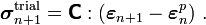
Part 12

In the radial return algorithm, we define a trial elastic state as

\text{(2)} \qquad \boldsymbol{\sigma}_{n+1}^{\text{trial}} = \boldsymbol{\sigma}_n + \boldsymbol{\mathsf{C}}:(\boldsymbol{\varepsilon}_{n+1} - \boldsymbol{\varepsilon}_n)

where $\boldsymbol{\sigma}_n,\boldsymbol{\varepsilon}_n$ are the stress and strain at $t = t_n$ and $\boldsymbol{\sigma}_{n+1},\boldsymbol{\varepsilon}_{n+1}$ are the values at $t = t_{n+1}$ . Show that, if the elastic response of the material is linear, equation (2) can be written as

\text{(3)} \qquad \boldsymbol{\sigma}_{n+1}^{\text{trial}} = \left[\lambda~\text{tr}(\boldsymbol{\varepsilon}_{n+1})~\boldsymbol{\mathit{1}} + 2\mu~\boldsymbol{\varepsilon}_{n+1}\right] - \left[\lambda~\text{tr}(\boldsymbol{\varepsilon}_n^p)~\boldsymbol{\mathit{1}} + 2\mu~\boldsymbol{\varepsilon}_n^p\right] ~.

Hint: Start by showing that

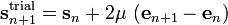
\boldsymbol{\sigma}_{n+1}^{\text{trial}} = \boldsymbol{\mathsf{C}}:(\boldsymbol{\varepsilon}_{n+1} - \boldsymbol{\varepsilon}_n^p) ~.

Part 13

Starting from equation (3) show that

\mathbf{s}_{n+1}^{\text{trial}} = \mathbf{s}_n + 2\mu~(\mathbf{e}_{n+1}-\mathbf{e}_n)

where $\mathbf{s}$ is the deviatoric part of $\boldsymbol{\sigma}$ and $\mathbf{e}$ is the deviatoric part of $\boldsymbol{\varepsilon}$ .

Part 14

Show that

\mathbf{s}_{n+1} = \mathbf{s}_{n+1}^{\text{trial}} - 2\mu~\Delta\gamma~\mathbf{n}_n ~.

Hint: The stress $\boldsymbol{\sigma}_{n+1}$ is given by

\boldsymbol{\sigma}_{n+1} = \boldsymbol{\mathsf{C}}:\boldsymbol{\varepsilon}_{n+1}^e ~.

Express this equation in terms of $\boldsymbol{\varepsilon}_{n+1}$ and $\boldsymbol{\varepsilon}_{n+1}^p$ . Then use the discretized equation for $\dot{\boldsymbol{\varepsilon}}^p$ (part 10) and the relation for $\boldsymbol{\mathsf{C}}$ for isotropic elasticity. Finally compute the deviatoric stress terms after showing that

\text{tr}(\mathbf{s}) = 0 ~.

Part 15

The discretized form of the Kuhn-Tucker conditions in conjunction with the consistency condition gives us

f(\boldsymbol{\sigma}_{n+1},\alpha_{n+1},T_{n+1}) = 0 ~.

Use this condition and the relations you have derived in the previous sections to arrive at a nonlinear equation in $\Delta\gamma$ that can be solved using Newton iterations.

Part 16

Let the nonlinear equation be $g(\Delta\gamma)$ . Recall that the Newton method requires that we iterate using the formula

\Delta\gamma_{r+1} = \Delta\gamma_r - \cfrac{g(\Delta\gamma_r)} {\cfrac{dg(\Delta\gamma_r)}{d\Delta\gamma}}

where $r$ is the Newton iteration number. Derive an expression for the derivative of $g$ that is required in the above formula.

(You can use Computational Inelasticity by J.C. Simo and T.J.R. Hughes for pointers.)

Problem 2: Billet Upset Forging

Consider the isothermal upset forging of the cylindrical billet shown in Figure 2.

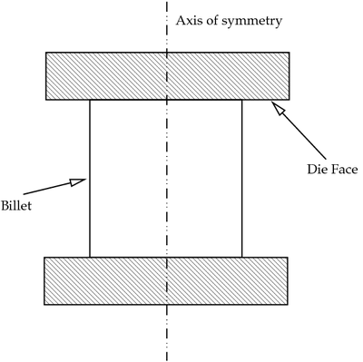Figure 2. Upset forging of a cylindrical billet.

Assume that the dies are rigid. Also assume that sticking friction is in effect between the billet and the die faces when they are in contact.

The billet has an initial radius of 10 mm and its initial height is 30 mm. The shear modulus of the material is 384.6 MPa, the bulk modulus of the material is 833.3 MPa, the initial yield stress is 1 MPa and the linear hardening modulus is 3 MPa.

Model a quarter of the cylinder using symmetry boundary conditions.

Apply a compressive force of 1 kN to the die.

Plot the final shape of the billet. Compare your results with those shown in Simo and Hughes (Fig. 9.8, p. 325).
Plot a curve of the die force (kN) versus the die stroke (mm). Compare your results with those shown in Simo and Hughes. Do you observe any volumetric locking?

(Use an implicit software to solve these problems.)

Problem 3: Taylor Impact Tests

Consider the impact of a cylindrical Taylor impact specimen on a rigid target. The undeformed and deformed profiles of the specimen are shown in in Figure 3.

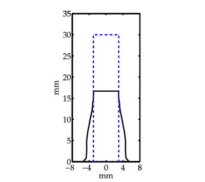Figure 3. Taylor impact test of a cylindrical rod.

The initial length of the specimen is 30 mm. The initial diameter is 6 mm. The initial velocity is 188 m/s. The initial temperature is 718 K.

The material of the specimen is OFHC copper. The properties of the bar are (in SI units):

Density	8930.0
Thermal conductivity	386.0
Specific heat	414.0
Shear modulus	46.0e9
Bulk modulus	129.0e9
Coeff. Thermal Expansion	1.76e-5

The plastic deformation of the specimen is described by the Johnson-Cook model and $J_2$ plasticity. The Johnson-Cook model parameters are (in SI units):

A	90.0e6
B	292.0e6
C	0.025
n	0.31
m	1.09
$\dot{\varepsilon_{}}_0$	1.0
$T_r$	294.0
$T_m$	1356.0

Use LS-DYNA to simulate the Taylor impact test. Assume that there is no friction between the anvil and the specimen. Plot the final deformed shape of the specimen and compare that with the experimentally determined shape given in the table below. What differences do you observe and why?

Point	x (mm)	y (mm)
1	0.000000	0.000000
2	5.436409	0.000000
3	4.711554	0.852540
4	4.611804	2.040725
5	4.581879	3.228910
6	4.615129	4.141866
7	4.585204	4.980980
8	4.448878	6.175878
9	4.312552	7.223092
10	4.073150	8.344149
11	3.870324	9.465205
12	3.597672	10.868203
13	3.388196	11.707317
14	3.218620	12.902215
15	3.152120	13.949429
16	2.982544	15.070486
17	2.952618	16.674871
18	0.000000	16.674871
19	0.000000	0.000000

You can generate a mesh in ANSYS and tranfer it to LS-DYNA if you want.

Show whether energy is conserved during your simulation.

This article is issued from Wikiversity - version of the Tuesday, January 08, 2008. The text is available under the Creative Commons Attribution/Share Alike but additional terms may apply for the media files.